Calibration of visually guided reaching is driven by error-corrective learning and internal dynamics

Abstract

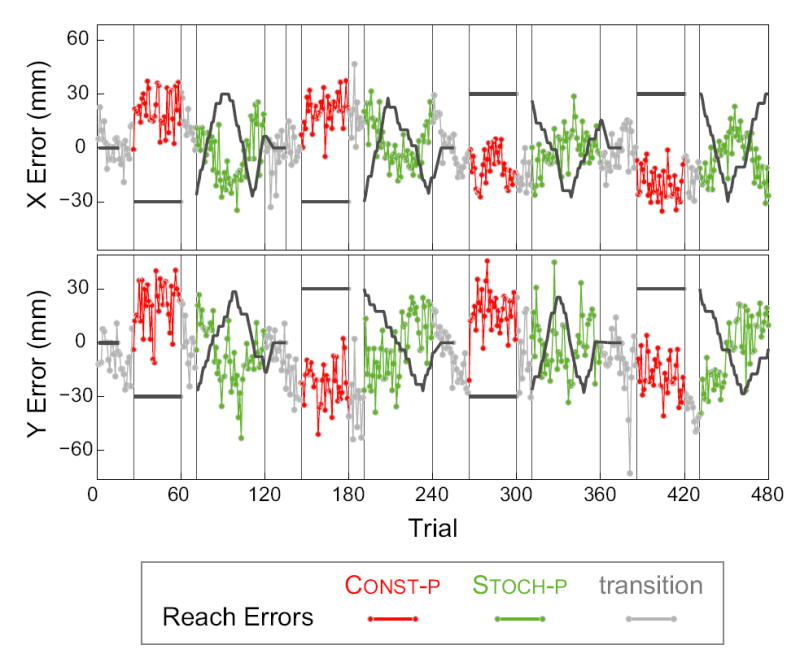
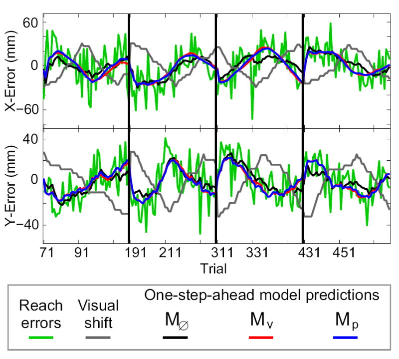
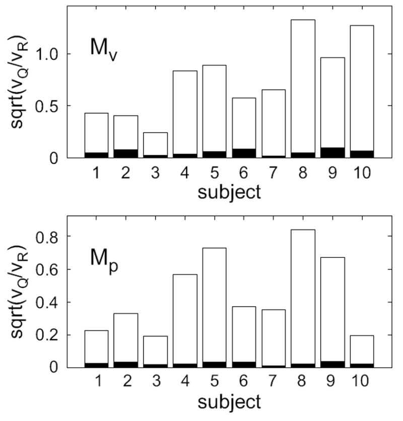
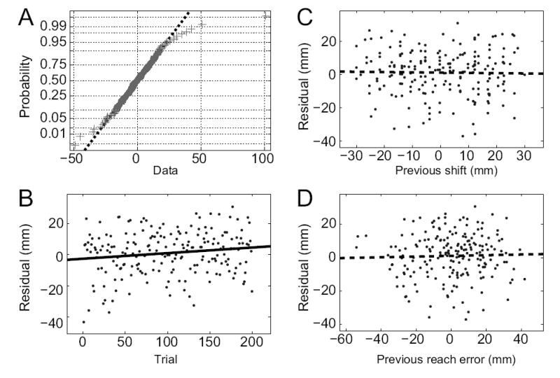
The sensorimotor calibration of visually guided reaching changes on a trial-to-trial basis in response to random shifts in the visual feedback of the hand. We show that a simple linear dynamical system is sufficient to model the dynamics of this adaptive process. In this model, an internal variable represents the current state of sensorimotor calibration. Changes in this state are driven by error feedback signals, which consist of the visually perceived reach error, the artificial shift in visual feedback, or both. Subjects correct for > or =20% of the error observed on each movement, despite being unaware of the visual shift. The state of adaptation is also driven by internal dynamics, consisting of a decay back to a baseline state and a "state noise" process. State noise includes any source of variability that directly affects the state of adaptation, such as variability in sensory feedback processing, the computations that drive learning, or the maintenance of the state. This noise is accumulated in the state across trials, creating temporal correlations in the sequence of reach errors. These correlations allow us to distinguish state noise from sensorimotor performance noise, which arises independently on each trial from random fluctuations in the sensorimotor pathway. We show that these two noise sources contribute comparably to the overall magnitude of movement variability. Finally, the dynamics of adaptation measured with random feedback shifts generalizes to the case of constant feedback shifts, allowing for a direct comparison of our results with more traditional blocked-exposure experiments.

FIG. 1

A: Virtual feedback setup. B: Definition of reach and feedback variables: f, location of unseen fingertip location at end of reach; c, location of visual feedback (cursor); g, target location; e, true reach error; υ, visually perceived reach error; p, artificial feedback shift (perturbation).

FIG. 2

An example trial sequence. Visual feedback shifts (black traces) and reach errors (see key at bottom) along the X-axis (top panel) and Y-axis (bottom panel) are shown. Gray vertical bars mark boundaries between blocks of trial types: Stoch-p: stochastically shifted feedback; Const-p: constant feedback shift; transition: trials include reaches without visual feedback to prevent subjects from noticing onset of constant shift blocks and ramping down of shift after a Stoch-p block.

FIG. 3

Hierarchical model selection. Arrows represent comparisons between nested model classes (boxes) made with the likelihood ratio test (LRT) on Stoch-p data. Each test had four degrees-of-freedom, corresponding to 2×2 matrix parameters. p-values for the LRT, shown next to the appropriate arrow, apply across all 10 subjects and were highly consistent. Thick lines represent comparisons for which the additional input variable resulted in a significant improvement

FIG. 4

Maximum likelihood LDS model parameters. Best fit parameters for the M_υ and M_p models. Each panel represents the values of a 2 × 2-matrix parameter (see label on y-axis), with values for all subjects clustered by the matrix component: $\left[\begin{array}{cc}11& 22\\ 21& 22\end{array}\right]$. Bar colors correspond to subjects (n = 10).

FIG. 5

Sample model predictions. Reach errors and one-step-ahead model predictions for one subject in the Stoch-p trial blocks.

FIG. 6

The linear dynamical system (LDS) model is sufficient to predict the statistical structure of the adaptive response to shifted feedback. A: Comparison of empirical reach error variance ${\sigma }_e^2$ and the predicted variance under the best-fit M_υ (black), M_p (green), and M_0̸ (red) models. Datapoints represent values for a single subject (symbols overlap), and thick lines represent a linear regression of empirical data on prediction (p < 0.05). B: Reach error auto-correlation function ρ_e (τ) for time lags τ = 1–8 trials. The dark gray band represents mean ± sem. across subjects. Model predictions are shown in three lines representing mean ± sem. across subjects: M_υ, green; M_p, black; M_0̸ red. C: Comparison of empirical values and model predictions of the covariance σ_ep between reach errors and visual shifts. Symbols as in A. D: Cross-correlation function ρ_ep (τ) between reach errors and feedback shifts, along with the Monte Carlo model predictions. Symbols as in B. E: Sensitivity analysis: how predicted cross-correlation functions depend on model parameters. The gray band (data) green line (M_υ model predictions) are the same as those in panel B. The other colored lines represent the cross-correlations predicted by the best-fit M_υ model with selected parameters altered, as indicated by the legends. Only the diagonal elements of the parameter matrices A and B were varied, while in the case of Q and R the entire matrix was scaled.

FIG. 7

Magnitude of estimated state noise relative to output noise (open bars) for two model classes fit to the Stoch-p data. υ_Q and υ_R are the largest eigenvalues of the state and output noise covariances, respectively. Filled bars represent the 95% confidence value under the null hypothesis of negligible state noise determined from 1000 Monte Carlo simulations.

FIG. 8

Comparison of empirical and predicted steady states of adaptation. Predictions were derived from the M_υ (•, solid lines) and the M_p (◦, dashed lines) models fit to Stoch-p data. Empirical values were averaged over the last 10 trials of each Const-p trial block. A: Magnitude of the steady state of adaption with a 30 cm magnitude shift along each axis. Empirical values are averages of the x and y error coordinates. The expression for model predictions is given in Cheng and Sabes (2006). Linear regression of the measured values on the model fits shown in bold lines (M_υ: R² = 0.52, p = 0.02; M_p: R² = 0.50, p = 0.02). B: Standard deviation of the reach error during steady state ( ${\sigma }_e^2$ in Eqn. 3a). Model predictions come from Monte Carlo simulations (see Methods). Linear regression in bold lines (M_υ: R² = 0.79, p = 0.007; M_p: R² = 0.81, p = 0.006).

FIG. 9

The dynamics model identified from Stoch-p data can also account for adaptation to constant visual shift. Plotting convention is the same as in Fig. 6. A: Reach errors variance vs. Monte Carlo model predictions. B: Auto-correlation function of reach errors for time differences of 1–8 trials and Monte Carlo model predictions. C: Covariance between reach errors and feedback shifts for individual subjects vs. Monte Carlo model predictions. Linear regression of subject data on model prediction was marginally significant: p = 0.06 for the M_υ model (green circles and green regression line) and p = 0.07 for the M_p model (black circles, thick black regression line). D: Cross-correlation function between reach errors and feedback shifts for time differences of 1–8 trials, along with the Monte Carlo model predictions. E: Sensitivity analysis of how predicted cross-correlation functions depend on model parameters.

FIG. 10

Examples of statistical analyses performed on the model prediction errors. A: Normal probability plot for the only residual component (x-component, Subject 8) that showed significant deviations from normality (N=199, Lilliefors test, p = 0.04). Data-points are represented by crosses; Gaussian data fall on a straight line (best fit line displayed as dashed line). Without the single large outlier (top-right of graph), the deviation from the Gaussian distribution is not significant (p > 0.2). B: Example of significant non-stationarity (linear regression, F-test, p = 0.036) in the model-fit residual (y-component, Subject 1). C,D: Example plots of model-fit residual (y-component, Subject 1) vs. visual shift on the prior trial (C) or reach error on the prior trial (D). Linear regression shows no significant effect in either plot (F-test, p = 0.79 and p = 0.69) and no clear non-linear relationships are discernible.

References

1. Anderson BDO, Moore JB. Optimal Filtering. Prentice-Hall; Englewood Cliffs, N.J: 1979.
1. Atkeson CG, Hollerbach JM. Kinematic features of unrestrained vertical arm movements. J Neurosci. 1985;5(9):2318–30. - PMC - PubMed
1. Baddeley RJ, Ingram HA, Miall RC. System identification applied to a visuomotor task: Near-optimal human performance in a noisy changing task. J Neurosci. 2003;23(7):3066–3075. - PMC - PubMed
1. Baizer JS, Glickstein M. Proceedings: Role of cerebellum in prism adaptation. J Physiol. 1974;236(1):34P–35P. - PubMed
1. Baizer JS, Kralj-Hans I, Glickstein M. Cerebellar lesions and prism adaptation in macaque monkeys. J Neurophysiol. 1999;81(4):1960–1965. - PubMed
Publication types
LinkOut - more resources