Part 1. Automated change detection and characterization in serial MR studies of brain-tumor patients

Abstract

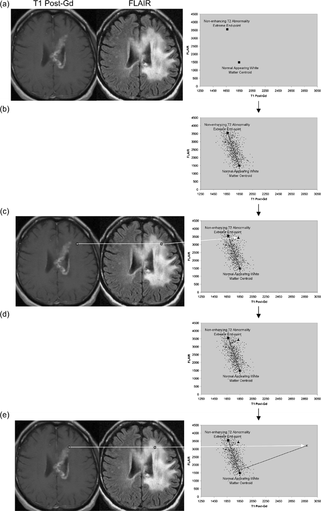
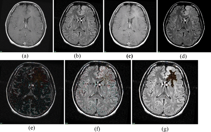
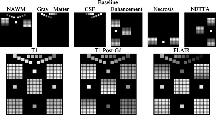
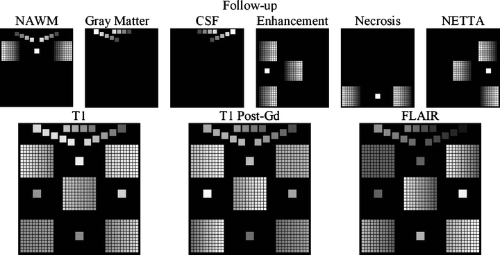
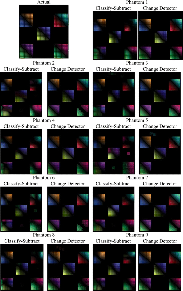
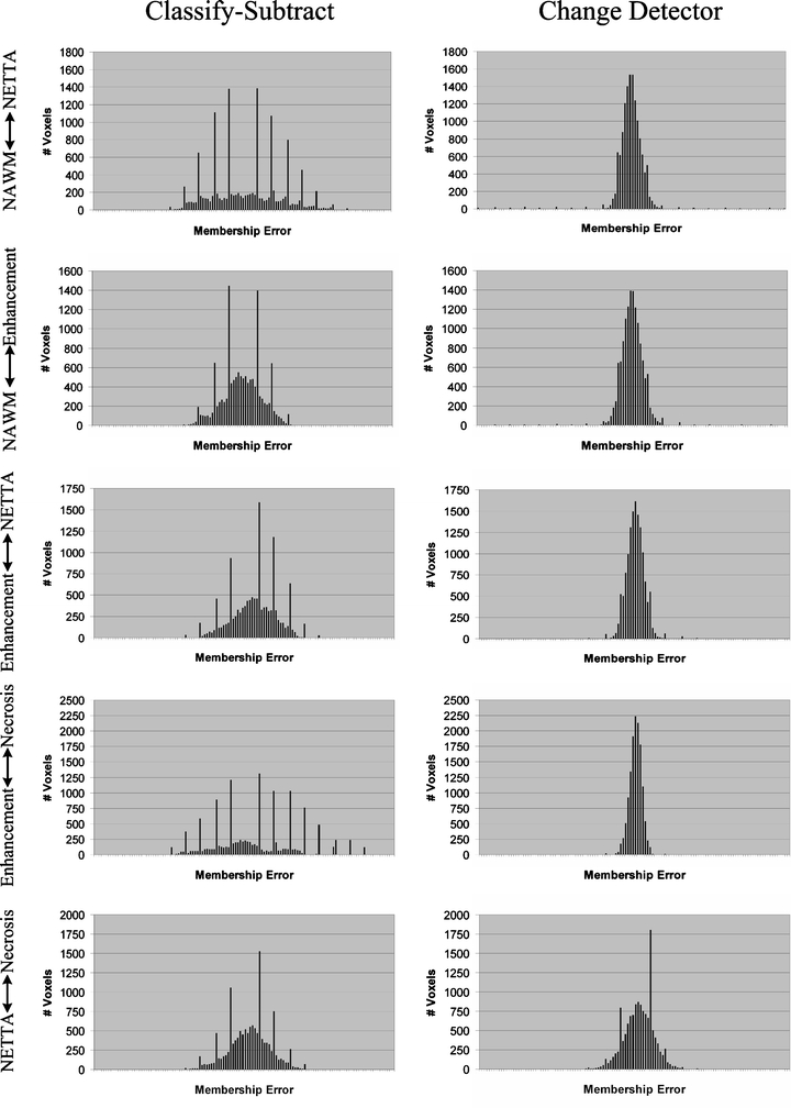
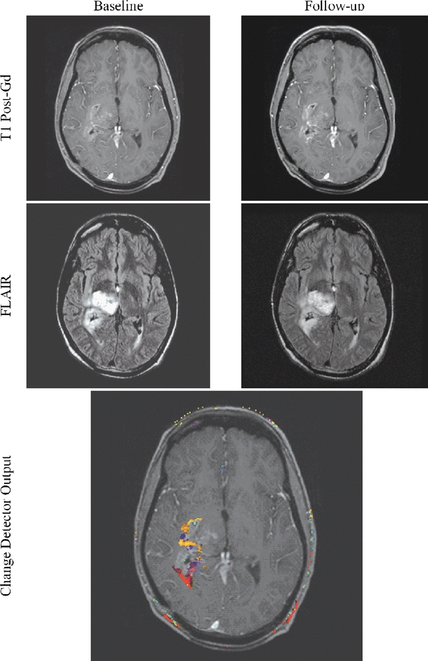
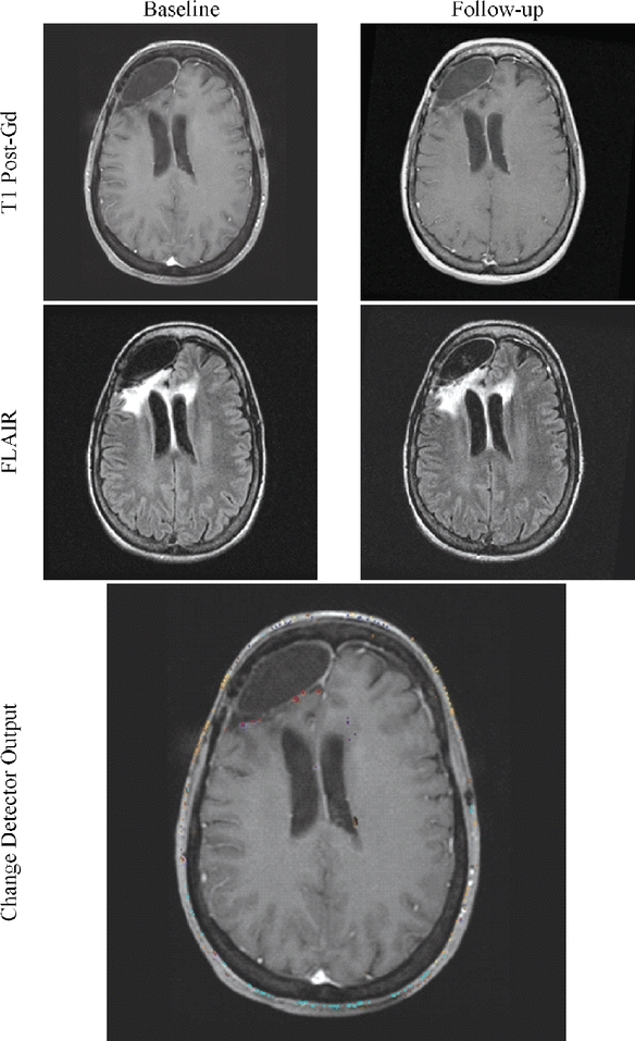
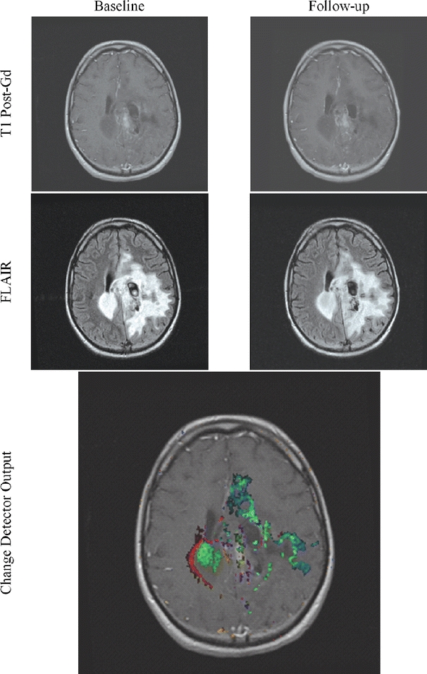
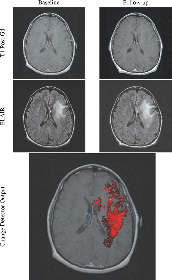
The goal of this study was to create an algorithm which would quantitatively compare serial magnetic resonance imaging studies of brain-tumor patients. A novel algorithm and a standard classify-subtract algorithm were constructed. The ability of both algorithms to detect and characterize changes was compared using a series of digital phantoms. The novel algorithm achieved a mean sensitivity of 0.87 (compared with 0.59 for classify-subtract) and a mean specificity of 0.98 (compared with 0.92 for classify-subtract) with regard to identification of voxels as changing or unchanging and classification of voxels into types of change. The novel algorithm achieved perfect specificity in seven of the nine experiments. The novel algorithm was additionally applied to a short series of clinical cases, where it was shown to identify visually subtle changes. Automated change detection and characterization could facilitate objective review and understanding of serial magnetic resonance imaging studies in brain-tumor patients.

Fig 1

Preprocessing.

Fig 2

Change detection algorithm.

Fig 3

A feature extraction step is performed, which recombines the original volumes to create a volume for each tissue pair at each acquisition. Each of these recombined volumes will be referred to as a transition-emphasizing extraction product (TEEP). This process of feature extraction is accomplished by casting a line through the centroids of each relevant pair of tissues, and then perpendicularly projecting all points in feature space onto the resulting line. (a) The intensities of voxels may be shown in a scatterplot. For clarity, a two-dimensional feature space made up of T1 and FLAIR is shown, but all three volumes (T1, T1 Post-Gd, and FLAIR) were used in this study. The intensities of two selected points from the volume are plotted here to demonstrate a voxel containing moderate NETTA (lower point), and another voxel containing more pronounced NETTA (upper point). The line in feature space connecting the centroid of NETTA with the NAWM centroid is also shown, as are the centroids of these tissues. (b) The feature extraction is accomplished by projecting all voxels onto the line connecting the NAWM and NETTA centroids using equation 1. (c) The output volume, or TEEP, is thus produced for each tissue-pair and acquisition. Note that the values on the line have been shifted to the right by 0.82 in order to ensure that the lowest-valued voxel in the TEEP as a whole will be exactly 0.0. In the case shown, the TEEP appears similar to the FLAIR image because most of the contrast between NAWM and NETTA is held in the FLAIR image. Voxels that are not either NETTA or NAWM will be removed from consideration of NETTA–NAWM transition in a later step (not shown in this figure). (d) The TEEP represents both tissues in a tissue pair; this may be shown more clearly by converting the values in the TEEP volume to two membership volumes using equation 2. This process is shown graphically for the more anterior of the two points in Figure 4.

Fig 4

Computing fractional membership from TEEPs. The line shown in the above figure corresponds to the NAWM↔NETTA TEEP from Figure 3c, and the point marked “x” corresponds to the more anterior of the two sample points. Within a given TEEP, the fractional membership is determined by the relative linear fractional distance from either end point. A voxel exactly on top of the NETTA end point would possess 1.0 membership in NETTA and 0.0 membership in NAWM, whereas the voxel situated at the marker shown would possess a membership of 0.7 in NETTA and 0.3 in NAWM. The symbols x, μ_A, and μ_B are provided for correspondence with equation 2.

Fig 5

Computation of the transaxial Mahalanobis distance. As in Figure 3a, the end points of the line corresponding to the NAWM↔NETTA dual-tissue pair, which were derived from part 1 of the algorithm, may be plotted. (b) Based upon the samples of NAWM and “extreme” NETTA, the algorithm synthesizes sample points following the line connecting the two centroids but offsets by noise. These represent the locations in the scatterplot where the algorithm would expect to find real NETTA possessing varying degrees of T2 abnormality. (c) The location of one particular voxel of real NETTA, drawn from the images, is shown in the scatterplot for demonstration purposes. Its location on the scatterplot, as expected, falls within the range of the synthesized NETTA points. (d) The line originating from this point which is perpendicular to the NAWM↔NETTA partial membership line is determined. The inverse of the square of the Mahalanobis distance from the point to its perpendicular projection on the NAWM↔NETTA partial membership line is determined using equation 3. When points are members of a given dual-tissue class, this inverse of the Mahalanobis distance should be low (roughly speaking, within the range of the inverse of the Mahalanobis distance for NAWM↔NETTA points shown; however, description of the precise mechanism of thresholding is beyond the scope of this article). (e) The location of one particular real voxel containing enhancing tissue (i.e., definitively not a member of the NAWM↔NETTA dual-tissue class) is shown, and this point’s multispectral intensity is plotted on the scatterplot. As in step (d), the line which originates from this point and which is perpendicular to the NAWM↔NETTA partial membership line is determined. The inverse square of the Mahalanobis distance between the point and its perpendicular projection onto the NAWM↔NETTA partial membership line is again determined using equation 3. When points are not members of a given dual-tissue class, the inverse square of the transaxial Mahalanobis distance is high.

Fig 6

Relationship between the number of voxels in a given region the and standard deviation multiplier used by the spatially adaptive noise reduction routines. Smaller regions are required to possess a higher mean change than larger regions in order to be considered to be due to an underlying biological process and not due to noise. In the figure, “σ” is specific to the dual-tissue class in question and is determined by how much static voxels belonging to that partial membership line vary. Note that if the region of spatial coherence is sufficiently large, a mean change well below the noise floor will be correctly identified as real. The actual form of the threshold was determined empirically; more statistically rigorous approaches are possible.

Fig 7

The color scheme used for all change detection images in this article. The color indicates the type of transition occurring, whereas the intensity indicates the size of change. Note that two colors correspond to each dual-tissue class because a change may proceed in either direction, e.g., previously, NAWM may develop increased enhancement (orange), and tissue which was already enhancing may also lose enhancing character (light blue, extreme upper left).

Fig 8

A sample change detection image, demonstrating the detection of changes which are subtle but which involve a large area. (a) T1 Post-Gd Time 0, (b) FLAIR Time 0, (c) T1 Post-Gd Time 1, (d) FLAIR Time 1, (e) Unthresholded color change map (which is dark because the change, while omnipresent, is of quite small membership). (f) Simple thresholded color change map, (g) adaptive thresholded change map. Note that the simple threshold has completely missed the change, but has not removed all noise, whereas the adaptive threshold technique eliminates virtually all noise and retains a large region of subtle change. The color scheme is shown in Figure 7; the region shown consists of an area of development of subtle enhancement.

Fig 9

Construction of the baseline change phantom. The membership volumes for the desired phantom (top row) are used in conjunction with intensity samples derived from patient brain images (not shown) to generate the synthetic pulse sequences (bottom row). The largest squares show regions of pure tissues, all of which can be seen to be invariant in terms of membership from the baseline to the follow-up scan. The medium-sized squares contain mixtures of normal tissues, all of which also can be seen to possess invariant membership mixtures from one time point to the next. Each of the five grids contains mixtures of pathological tissues, with each grid corresponding to one of the dual-tissue classes.

Fig 10

Construction of the follow-up change phantom. As in Figure 9, the membership volumes for the desired phantom (top row) are used to generate the synthetic pulse sequences (bottom row). Note the difference in orientation of the gradation within the grids at each time point. The result is a broad range of starting and stopping membership values over each grid/dual-tissue class.

Fig 11

Ground truth output for the change detection phantom (upper left), and output for both the classify–subtract and the change detection algorithms for all nine serial phantoms.

Fig. 12

Histograms of errors for phantom 1 over each dual-tissue class. The x-axis labels (membership error) range from −1 to +1 for all charts, with the bin corresponding to zero error located at the center of each chart. The ideal histogram would be one in which there was a single bar in the center of each histogram, signifying that all voxels possessed zero error. The distributions of errors for the change detector appear more regular, Gaussian, and are centered on error=0.0 in all cases. The distributions of errors for the classify–subtract algorithm appear broader with bins located further from the center, signifying a greater number of voxels with larger error. The graphs corresponding to the classify–subtract algorithm additionally possess many large spikes, corresponding to voxels where the classify–subtract algorithm failed to correctly identify the dual-tissue class of voxels (the discreteness of these spikes results from the discreteness of the phantom’s underlying bins).

Fig 13

Subtle but important changes may hide in and around a lesion. The algorithm possesses the ability to identify and highlight such subtle changes.

Fig 14

Confirmation of stability can be as difficult as the detection of change. The change detector’s ability to reject noise can help confirm the patient’s unchanging status.

Fig 15

Change may be difficult to interpret because of the complexity of the lesion. Use of the change detector lessens this difficulty.

Fig 16

Change may be subtle in parts but more dramatic when taken as a whole.

References

1. Simons DJ, Levin DT. Change blindness. Trends Cogn Sci. 1997;1:261–267. doi: 10.1016/S1364-6613(97)01080-2. - DOI - PubMed
1. Rensink RA. Change detection. Annu Rev Psychol. 2002;53:245–277. doi: 10.1146/annurev.psych.53.100901.135125. - DOI - PubMed
1. Patriarche J, Erickson B. A review of the automated detection of change in serial imaging studies of the brain. J Digit Imaging. 2004;17:158–174. doi: 10.1007/s10278-004-1010-x. - DOI - PMC - PubMed
1. Radke RJ, Andra S, Al-Kofahi O, Roysam B. Image change detection algorithms: a systematic survey. IEEE Trans Image Process. 2005;14:294–307. doi: 10.1109/TIP.2004.838698. - DOI - PubMed
1. Miller AB, Hoogstraten B, Staquet M, Winkler A. Reporting results of cancer treatment. Cancer. 1981;47:207–214. doi: 10.1002/1097-0142(19810101)47:1<207::AID-CNCR2820470134>3.0.CO;2-6. - DOI - PubMed
Publication types