Efficient classification of complete parameter regions based on semidefinite programming

Abstract

Background: Current approaches to parameter estimation are often inappropriate or inconvenient for the modelling of complex biological systems. For systems described by nonlinear equations, the conventional approach is to first numerically integrate the model, and then, in a second a posteriori step, check for consistency with experimental constraints. Hence, only single parameter sets can be considered at a time. Consequently, it is impossible to conclude that the "best" solution was identified or that no good solution exists, because parameter spaces typically cannot be explored in a reasonable amount of time.

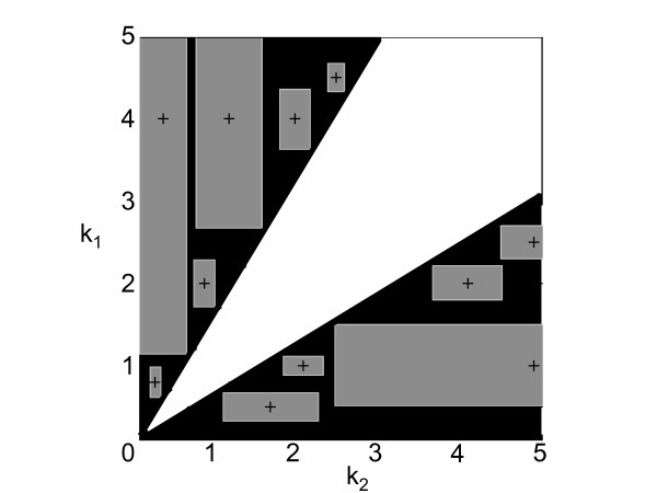
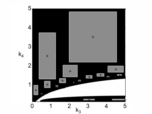
Results: We introduce a novel approach based on semidefinite programming to directly identify consistent steady state concentrations for systems consisting of mass action kinetics, i.e., polynomial equations and inequality constraints. The duality properties of semidefinite programming allow to rigorously certify infeasibility for whole regions of parameter space, thus enabling the simultaneous multi-dimensional analysis of entire parameter sets.

Conclusion: Our algorithm reduces the computational effort of parameter estimation by several orders of magnitude, as illustrated through conceptual sample problems. Of particular relevance for systems biology, the approach can discriminate between structurally different candidate models by proving inconsistency with the available data.

Figure 1

Graph of the feasible parameter space. Contour plot of the three-dimensional parameter space of k₁, k₂ and k₃ from the example given in the text. The cone with the black edges marks the feasible region, infeasible areas are illustrated as cuboids with gray edges. Gray circles represent the original set of parameters where the bisection search started.

Figure 2

Maximal possible parameter perturbation. The size η of the maximal possible perturbation in the example given in the text is shown as a function of k₁ and k₃ (here, k₂ = 1). The size of the perturbation increases with the distance from the feasible region and can be used to further refine the search directions in parameter space.

Figure 3

Uncertain model structure. It is unknown whether A exerts a positive influence on the conversion of B to D. By numerical integration of model alternative II, concentrations were obtained and used in lieu of experimental data. Overall component concentrations, a step response upon an increase of v₁ and corresponding steady states (circle) are indicated in the inlays next to each component.

Figure 4

Model discrimination based on two distinct steady states. The figure shows variations in v₁ simulated with model I (gray dashed line) and model II (black solid line), respectively. A large standard deviation of the experimental data (ε = 0.75, dashed error bars) has to be allowed for model I, otherwise mass balances are violated (ε = 0.25, solid error bars). For the simulations, the constants for complex formation were set to the following values: association k_on,i = 1; dissociation k_off = 0.1; catalytic step k_cat,i = 1. During the parametrization step, only the association constants of the complexes were estimated in a range from 0.3 to 3.

Figure 5

Contour plot for additional example 1. The feasible and infeasible regions are shown in white and black, respectively. Starting from an initial set of parameters (black cross), whole areas can be proven to be inconsistent (gray).

Figure 6

Contour plot for additional example 2. The feasible and infeasible regions are shown in white and black, respectively. Starting from an initial set of parameters (black cross), whole areas can be proven to be inconsistent (gray) (parameters k₁ and k₂ are fixed, k₃ and k₄ are varied in a range between 0 and 5).