The mechanics of active fin-shape control in ray-finned fishes

Abstract

We study the mechanical properties of fin rays, which are a fundamental component of fish fin structure. We derive a linear elasticity model that predicts the shape of fin rays, given the input muscle actuation and external loading. We then test the model using experiments that measure (i) the ray deflection for a given actuation at the muscular interface, and (ii) the force-displacement response under conditions of actuation and non-actuation. The model agrees well with the experiment; both show a concentration of curvature at the ray base or at the point of an externally applied force, and a variation in ray stiffness over more than an order of magnitude depending on actuation at the bases of the fin rays.

Figure 1

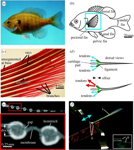
(a) A photograph of a bluegill sunfish. (b) Schematic showing the location of the fish fins. The pectoral fin is highlighted with the blue box. (c) A photograph of a cleared and stained pectoral fin. The short segments can be seen along the length of the rays. (d) Schematic showing dorsal views of a fin ray with two hemitrichs. Muscles (not shown) exert forces on the tendons attached to the head of each hemitrich. (e) Single cross-section slice from a microCT scan of a pectoral fin. The upper panel shows multiple rays and the lower panel shows an expanded cross-section of two rays. Each of the two rays is composed of two hemitrichs. The bright white regions are bony areas and the grey is softer tissues (fin membrane and connective tissues). The separation between the two hemitrichs of the left ray is labelled ‘dist=d’. (f) Apparatus for holding ray hemitrichs. The ray (label ‘i’) is held by two clips (label ‘ii’). The upper clip can move to apply an offset between the hemitrichs. The inset image shows the end-on view. The upper clip holds one hemitrich and the lower clip holds the other hemitrich.

Figure 2

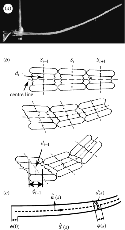
(a) A photograph of a single fin ray (ray 4 out of 13 in the pectoral fin of a bluegill sunfish) held by force calipers in the experimental set-up. The upper hemitrich base is displaced to the left relative to the lower hemitrich base, leading to an upward deflection. (b) A schematic of the physical mechanism of fin-ray bending proposed by Geerlink & Videler (figure adapted from the original figure in Geerlink & Videler 1987). We introduce here the notation s for the arc length along the ‘centre line’—the line at the average position of the initially opposite hemitrichia; d for the distance between midpoints of opposing segments; ϕ for the displacement of the segment in the direction tangent to the centre line. Subscripts denotes segment number i. (c) The model we consider in this work, which is the continuum limit of the diagram in (b).

Figure 3

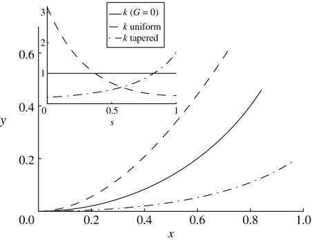
Three representative trajectories of the fin-ray model with a base shift of ϕ₀=0.01, where the undeflected ray (ϕ₀=0) lies along the x-axis: 1, a ray with zero shear modulus and fused end (equation (4.1); solid line); 2, a uniform ray (equation (4.3); dashed line); and 3, a ray with G increasing towards the end as 11s¹⁰, d linearly tapered as 0.02(1.5−s), and B=d³ (dashed-dotted line), intended to simulate the case of a tapered ray with shear modulus weighted towards the tip (see §4.1.3). Inset, the curvature as a function of arc length for the three cases. The curvature either decreases (dashed line), remains constant (solid line) or increases (dashed-dotted line) towards the end.

Figure 4

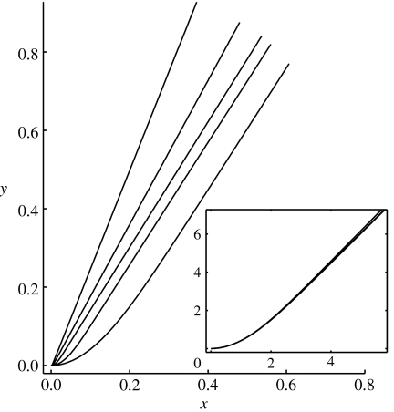
Solutions to the centre-line equation (3.14) for rays with uniform G varying over five orders of magnitude (10², 10³, 10⁴, 10⁵, 10⁶), and uniform intraray spacing (d=0.01), bending modulus (B=1) and base shift ϕ₀=0.01. Deflection increases with G. Inset, the five rays plotted with distances multiplied by $1/L_0=\sqrt{G/B}$, so the vertical axis shows $\sqrt{G/B}y$ and the horizontal axis shows $\sqrt{G/B}x$. The curves overlap closely. For large $\sqrt{G/B}$, L₀ is the size of the region at the base of the ray where bending is concentrated.

Figure 5

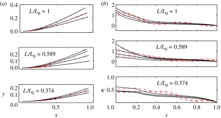
(a) A comparison between model (solid lines) and experimental (dashed-dotted lines) fin-ray trajectories. For each of the three ray fractions given in table 1, three to four trajectories are shown, each for a different base shift ϕ₀. The shear moduli used for the model are those which minimize the mean-square distance between the trajectories and are given in the third column of table 1. (b) Experimental and model fin-ray curvatures (κ) versus arc length (s) for the same datasets. The shear moduli used for the model are those which minimize the mean-square difference between the curvatures and are given in the fourth column of table 1.

Figure 6

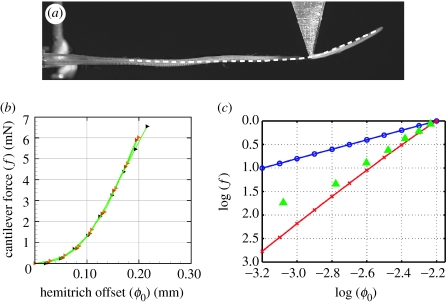
(a) A comparison between the model (dashed line) and the experimental trajectory (photograph), when a point force is applied (aluminium triangle in the photograph) at two-thirds the distance from the base to the tip of the ray. The point s=0 for the model is defined as the point where both hemitrichs appear fully segmented in the photo, though here the agreement is relatively insensitive to where s=0 is defined, since the bending occurs mainly beyond the point force. (b) Experimental measurements of the force versus base shift, for a point force which holds a point two-thirds along the ray fixed as in (a). (c) The data in (b) replotted on a log–log scale (green triangles), together with the corresponding data for the two models: equation (3.14), a uniform-shear-modulus material (blue circles) showing a linear growth of force with shift, and equation (3.15), collagen springs (red crosses) showing a cubic growth of force with shift. Forces f have been normalized to the value 1 at ϕ₀=10^−2.2, and only the slopes of the lines are to be compared.

Figure 7

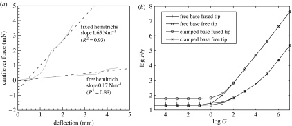
(a) The ability of the ray-shifting mechanism to resist a point force is quantified in the experiment by measuring the deflection of the ray versus an applied point force, for two different conditions at the base of the ray. The ray is clamped horizontally at the base, and a vertical point force is applied at two-thirds of the distance from the ray base to the tip, as in figure 6a. When only one of the bases is clamped, the ray deflects much more than when both bases are clamped. In the latter case, the force–displacement curve may be fit with a slope of 1.98 N m⁻¹, about 12 times the value when one hemitrich is free. Dashed lines show linear fits to the data. (b) In the corresponding model, only slopes of the corresponding curves in the linear (small-deflection) regime are shown, versus the non-dimensional shear modulus G (introduced in equation (3.11)). Four boundary conditions are tested—two at the base (both bases clamped versus one free) and two at the tip (hemitrichs fused or free at the tip). When G≪1, G drops out of the problem and the bending modulus B alone resists the force as a classical cantilever. In this limit, if the tip is fused, the resistance is increased. By contrast, for G≫1, the slope increases linearly with G in all cases, as the shear modulus provides the primary resistance. As G increases through 1, the ratio of force–displacement with both bases clamped versus one free transitions from 3 to 100; the experimental ratio of 12 occurs for G≈10², which is close to the values of G found by ray-shape fitting in table 1.

Figure 8

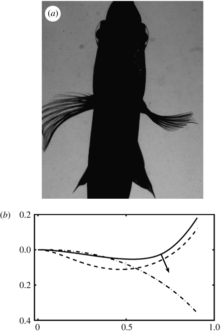
(a) Ventral view of a bluegill turning to the right. The fin to the right is actively cupped into the flow, increasing the drag force. (b) Shapes of a model fin ray under three loading situations: 1, a concentrated normal point load (solid line, equation (5.1) with ϕ₀=0.01=0.01, Q=220, d=0.01, G=200, B=1 and s₀=2/3); 2, a uniform force per unit length (dashed line, equation (5.1) with ϕ₀=0.01, p=200, d=0.01, G=200 and B=1); 3, a ‘passive’ ray under the same uniform loading (dashed-dotted line), with a free base (∂_sϕ=0 at s=0). The difference between 2 and 3 shows the effect of changing the base shift ϕ₀ from its passive value.

References

-
- Antman S.S. 2nd edn. Springer; New York, NY: 2005. Nonlinear problems of elasticity.
- Batchelor G.K. 1st edn. Cambridge University Press; Cambridge, UK: 1967. An introduction to fluid dynamics.
- Craven P, Wahba G. Smoothing noisy data with spline functions—estimating the correct degree of smoothing by the method of generalized cross-validation. Numerische Mathematik. 1979;31:377–403. doi: 10.1007/BF01404567. - DOI
- Geerlink P.J, Videler J.J. The relation between structure and bending properties of teleost fin rays. Neth. J. Zool. 1987;37:5980.
MeSH terms
LinkOut - more resources
Full Text Sources