Useful signals from motor cortex

Abstract

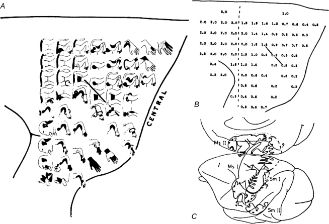
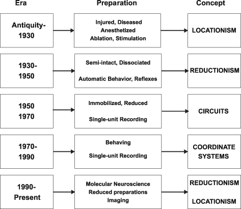
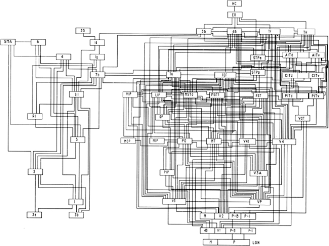
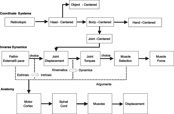
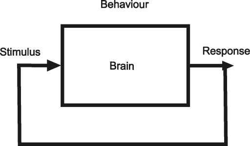
Historically, the motor cortical function has been explained as a funnel to muscle activation. This invokes the idea that motor cortical neurons, or 'upper motoneurons', directly cause muscle contraction just like spinal motoneurons. Thus, the motor cortex and muscle activity are inextricably entwined like a puppet master and his marionette. Recently, this concept has been challenged by current experimentation showing that many behavioural aspects of action are represented in motor cortical activity. Although this activity may still be related to muscle activation, the relation between the two is likely to be indirect and complex, whereas the relation between cortical activity and kinematic parameters is simple and robust. These findings show how to extract useful signals that help explain the underlying process that generates behaviour and to harness these signals for potentially therapeutic applications.

Figure 1

Delineation of motor cortex A, body movements resulting from 60 Hz AC stimulation of the motor cortical surface. B, stimulus intensities at which corresponding movements in A were just elicited. C, figurines created in primary and supplementary motor cortices from electrical stimulation as well as maps generated in primary and secondary sensory areas from peripheral stimuli. Figure from Clinton Woolsey published in Phillips & Porter (1977); reprinted with permission from Elsevier.

Figure 2

Historical description of neurophysiological investigation Interpretation presented using boxology.

Figure 3

Circuit diagram showing hierarchical organization of brain areas, arranged according to anatomical and receptive field properties Right side shows nodes of the visual system. Left side is for the somatosensory system. Modified from Van Essen, Anderson & Feldman (1991 used with permission).

Figure 4

Engineering boxology Top row shows a co-ordinate transformation scheme in which the target is sensed visually and the goal is represented in successive co-ordinate frames. Middle row shows inverse dynamics starting from a trajectory and ending with muscle force. Bottom row shows the anatomical schematic of output action.

Figure 5

Schematic diagram of brain and behaviour Closed-loop feedback generated from action that is sensed.

Figure 9

Different examples from Area 3b The method in Fig. 8 was used across a range of letters and different units.

Figure 8

Spatial event plot (from Phillips et al. 1988) An embossed drum was used to scan letters over the receptive field of a mechanoreceptor in a monkey's finger. Action potentials recorded from a single unit in Area 3b are registered on the plot as tick marks. The beginning of each row is aligned to the beginning of the scan and different rows correspond to successive vertical shifts of the drum over the finger. This method shows that an isomorphic replica of the letter ‘K’ can be recovered from the neural activity.

Figure 7

Linear encoding of mechanical stiumuli Plots of response versus intensity of mechanical stimulation. A shows responses from humans of estimated intensity of peripheral stimulus. B shows firing rate intensity of primary afferent in response to skin indentation. C shows post-central response to skin indentation. From Mountcastle (1984), used with permission.

Figure 6

Spike train recorded from mechanoreceptor afferent fibre Ordered up-to-down, left-to-right as successively greater displacement is imparted to the receptive field. From Mountcastle (1984), used with permission.

Figure 11

Tuned directional response This is an example of a unit response recorded during the centre-out task. Top panel shows rasters arranged by movement direction. Each row in the raster is a trial aligned to movement onset. The unit fired intensely for upper (90 deg) movements and slowed for the opposite downward movement. Firing intensity was graded for movements between these extremes. Bottom panel shows cosine tuning of cortical response. The data from the top panel are redisplayed as mean firing rates in each direction and these are fitted with a cosine. The peak of the cosine is near 90 deg and is termed the ‘preferred direction’. Reprinted with permission from Georgopoulos et al. (1982), copyright 1982 by the Society of Neuroscience.

Figure 10

Original centre-out model A monkey grasped the handle (‘C’) of a draftsman's arm and moved the sighting glass (‘D’) over a sequence of target lights embedded in the underlying table top. The sequence would begin with the capture of the centre target. This target would then be extinguished as one of the eight peripheral targets was illuminated, signalling the monkey to move towards and capture that target. Reprinted with permission from Georgopoulos et al. (1982), copyright 1982 by the Society of Neuroscience.

Figure 12

Decoding considerations Using a single tuning function to generate predicted movement direction does not work well because there are two directions for each discharge rate. This can be addressed by adding more units with different preferred directions and this combination will lead to a better solution (see text).

Figure 13

Population vector algorithm The response of each unit in a population during movements to each target is represented by a vector in that unit's preferred direction weighted (length) by the unit's firing rate during the movement. The vectors in each cluster are summed to give a resultant population vector (dashed arrow), which is predictive of movement direction. From Georgopoulos et al. (1983), with permission.

Figure 14

Neural trajectory Population vectors are made every 10–20 ms throughout a single drawing task. Monkeys used their fingers to trace a template on a touch monitor. The blue cluster is composed of preferred direction vectors, one from each cell recorded population. The population vectors (yellow example) in the sequence are connected tip-to-tail to construct a neural representation of the trajectory, which in this case is a spiral. This figure corresponds to Movie 4.

Figure 16

The projected object and cursor from the monkey's perspective

Figure 15

Virtual reality model Monkeys viewed images projected in stereo through a periscope. The resulting 3-D image appeared to be floating in front of them. Their hand position was tracked in 3-D and this was used to move a cursor ball in real time. The animals were trained to place the cursor in the tubular object and trace it.

Figure 19

Results of the illusion task Top row shows data collected from the primary motor cortex. The red trace represents the neural trajectory from M1, blue is the hand trajectory and green is the cursor path. The gain is changed in cycles 3–4, and both the neural and hand trajectories become circular. Bottom row shows neural trajectories from the ventral premotor cortex. These data show that the neural trajectory matches the cursor path instead of the hand trajectory. From Schwartz et al. (2004).

Figure 18

Motor illusion task Subjects drew five oval cycles in virtual reality. The top row shows what the hand did, starting from the first cycle, which uses normal gain, and proceeding through the subsequent cycles as the horizontal gain is increased to 1.8. The subject's hand trajectory became more circular throughout the task. The bottom row shows that the movement in the visual display of the cursor in the oval template continued to appear the same through the task.

Figure 17

Schematic of brain structures between primary visual and motor cortex MT, middle temporal; MST, medial superior temporal; VIP, ventral intraparietal; LIP, lateral intraparietal; Cing, cingulate; PMv, ventral premotor; PMd, dorsal premotor; M1, primary motor; AIT, anterior inferotemporal temporal; PN, pontine nuclei; Cb, cerebellum; SMA, supplementary motor; pSMA, presupplementary motor; and VPLo, ventral posterior lateral oralis (thalamus).

Figure 21

Power law When data from the figure of eight experiment were plotted as angular velocity versus curvature^−2/3, the relation was linear. This was true for both hand (top) and neural trajectories (bottom). From Schwartz & Moran (1999), used with permission.

Figure 20

Segmentation during drawing Monkeys were trained to draw four different figures of eight. Their finger trajectories (right column) were divided into four segments at points of maximum velocity. The same segmentation was found in the neural trajectories (left column). From Schwartz & Moran (1999), used with permission.

Figure 23

Density plot of the hand during ellipse drawing The hand slowed, spending more time, in the curves. The top of the color bar represents high probability.

Figure 22

Density plot of eye position during drawing The eyes tended to stabilize in either corner of the ellipse. The top of the color bar represents high probability.

Figure 24

Planar Michigan silicon array Photograph of a single multiprobe with four shanks, each containing four recording electrodes, displayed on the back of a penny. Courtesy of Dr Daryl Kipke, University of Michigan.

Figure 26

Plot of confidence intervalversusnumber of cells included in the population Using the method shown in Fig. 25, 95% confidence intervals (radius in degrees) were calculated for populations of different sizes in the 3-D centre-out task. The line with the boxes is for data calculated in a hand-control task (Georgopoulos et al. 1988). The continuous line is from the same task performed with brain-control.

Figure 25

Confidence interval of 3-D population vector A bootstrap technique was used to repeatedly calculate a population vector from its individual constituents. The results were rank ordered and represented as a 95% confidence interval around the mean population vector. This is represented by the radius of the red cone. The green vector is the movement vector for this 3-D centre-out example.

Figure 28

Robot trajectories towards the mouth Same explanation as for Fig. 26 for the opposite movements. The diameter of each target ball is 3 cm.

Figure 27

Robot trajectories during brain control Trajectories from the mouth to each of four food positions along with their 95% confidence intervals are shown for the initial self-feeding task. Once the gripper entered the target zone (solid balls), the arm moved automatically to the food. The diameter of each target ball is 3 cm.

References

1. Bernstein NA. The Coordination and Regulation of Movements. Oxford: Pergamon Press; 1967.
1. Evarts EV. Relation of pyramidal tract activity to force exerted during voluntary movement. J Neurophysiol. 1968;31:14–27. - PubMed
1. Felleman DJ, Van Essen DC. Distributed hierarchical processing in the primate cerebral cortex. Cereb Cortex. 1991;1:1–47. - PubMed
1. Ferrier D. Experiments on the brains of monkeys. Proc R Soc London (Biol) 1875;23:409–430.
1. Fitts PM, Denninger RL. S-R compatibility: correspondence among paired elements within stimulus and response codes. J Exp Psychol. 1954;48:483–492. - PubMed
LinkOut - more resources