. 2007 Feb 23:8:61.
doi: 10.1186/1471-2105-8-61.

Factor analysis for gene regulatory networks and transcription factor activity profiles

Affiliations

Factor analysis for gene regulatory networks and transcription factor activity profiles

Iosifina Pournara et al. BMC Bioinformatics. .

Abstract

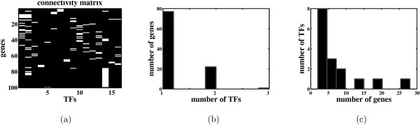
Background: Most existing algorithms for the inference of the structure of gene regulatory networks from gene expression data assume that the activity levels of transcription factors (TFs) are proportional to their mRNA levels. This assumption is invalid for most biological systems. However, one might be able to reconstruct unobserved activity profiles of TFs from the expression profiles of target genes. A simple model is a two-layer network with unobserved TF variables in the first layer and observed gene expression variables in the second layer. TFs are connected to regulated genes by weighted edges. The weights, known as factor loadings, indicate the strength and direction of regulation. Of particular interest are methods that produce sparse networks, networks with few edges, since it is known that most genes are regulated by only a small number of TFs, and most TFs regulate only a small number of genes.

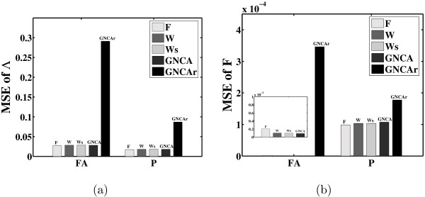
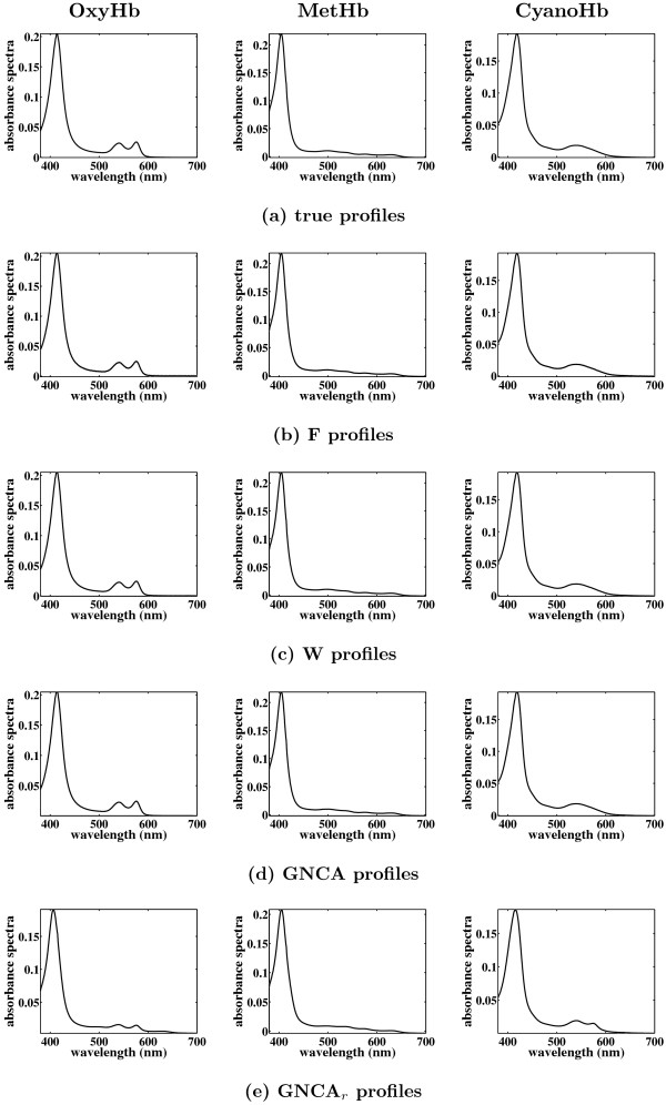
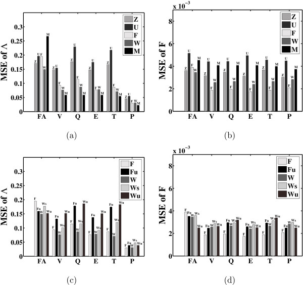
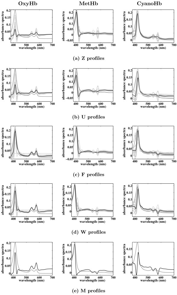
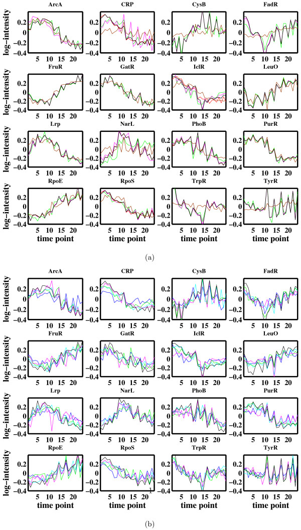
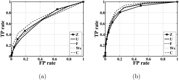
Results: In this paper, we explore the performance of five factor analysis algorithms, Bayesian as well as classical, on problems with biological context using both simulated and real data. Factor analysis (FA) models are used in order to describe a larger number of observed variables by a smaller number of unobserved variables, the factors, whereby all correlation between observed variables is explained by common factors. Bayesian FA methods allow one to infer sparse networks by enforcing sparsity through priors. In contrast, in the classical FA, matrix rotation methods are used to enforce sparsity and thus to increase the interpretability of the inferred factor loadings matrix. However, we also show that Bayesian FA models that do not impose sparsity through the priors can still be used for the reconstruction of a gene regulatory network if applied in conjunction with matrix rotation methods. Finally, we show the added advantage of merging the information derived from all algorithms in order to obtain a combined result.

Conclusion: Most of the algorithms tested are successful in reconstructing the connectivity structure as well as the TF profiles. Moreover, we demonstrate that if the underlying network is sparse it is still possible to reconstruct hidden activity profiles of TFs to some degree without prior connectivity information.


Figures

Figure 1
Figure 1
Factor loadings matrix of the E. coli network. (a) connectivity matrix of E. coli as suggested by Kao et al. [6] (a black entry corresponds to a non interaction while a white entry corresponds to an interaction), (b) distribution of the number of genes regulated by each TF, and (c) distribution of the number of TFs regulating each gene in the E. coli network of (a).
Figure 2
Figure 2
Distributions of genes and TFs for the simulated networks. The plots on the left hand side show the distribution of the number of genes regulated by each TF for three networks with densities 15, 25 and 40, respectively. The right hand side plots show the distribution of the number of TFs regulating each gene for the same networks.
Figure 3
Figure 3
Evaluation of the FA algorithms on E. coli simulated networks. Mean squared errors (MSEs) for Λ, the varimax rotated Λvari, and the procrustes rotated Λprocr are shown. The first column (a) shows the MSEs of Λ versus the network density, the second column (b) shows the MSEs of Λ versus the dataset size, and the third column (c) shows the MSEs of Λ for different values of the snr. These tests are for networks consisting of 50 genes and 8 TFs. Shown are the mean for 3 different networks. For the definition of the symbols M, Z, U, F, W and Ws see page 6.
Figure 4
Figure 4
Convergence test and processing time. (a) convergence test for the Gibbs sampling algorithms, and (b) the average time consumed by each algorithm.
Figure 5
Figure 5
Reconstruction of the factor loadings matrix for the Hemoglobin data. Mean square errors (MSEs) for (a) the factor loadings matrix Λ and (b) the factors matrix F. The positions of the zero entries in the loadings matrix are given a priori. FA stands for the output of a given FA algorithm. The procrustes (P) factor rotation method is applied to this output to indicate the performance of the algorithms when the best possible rotation is achieved.
Figure 6
Figure 6
Reconstruction of the factors matrix for the Hemoglobin data. Shown are (a) the true profiles of OxyHb, MetHb and CyanoHb, (b) the reconstructed profiles given by algorithm F, (c) the reconstructed profiles given by algorithm W, (d) the reconstructed profiles given by algorithm GNCA, and (e) the reconstructed profiles given by algorithm GNCAr. The positions of the zero entries in the loadings matrix are given a priori. The light gray curves are the profiles given by the 20 different Gibbs sampling runs, and the black curves are the average profiles. In these figures, the average profile of each factor coincides with its profile given by each single run.
Figure 7
Figure 7
Reconstruction of the factor loadings matrix for the Hemoglobin data. Mean square errors (MSEs) for (a) and (c) the factor loadings matrix Λ, and (b) and (d) the factors matrix F. The positions of the zero entries in the loadings matrix are not given a priori. FA stands for the output of a given FA algorithm. On this output, a number of factor rotation methods (varimax (V), quartimax (Q), equamax (E), tanh (T) and procrustes (P)) are evaluated based on the MSE. (c) and (d) show the performance of algorithms F and W under different priors regarding the loadings matrix (for further details see section Hemoglobin dataset).
Figure 8
Figure 8
Reconstruction of the factors matrix for the Hemoglobin data. Shown are (a) the reconstructed profiles given by algorithm Z, (b) the reconstructed profiles given by algorithm U, (c) the reconstructed profiles given by algorithm F, (d) the reconstructed profiles given by algorithm W, and (e) the reconstructed profiles given by algorithm M. The positions of the zero entries in the loadings matrix are not given a priori. The light gray curves are the profiles given by the 20 different Gibbs sampling runs, and the black curves are the average profiles. We also plot with gray the true profiles for an easier comparison. These profiles are obtained after performing varimax rotation on the factor loadings matrix.
Figure 9
Figure 9
Reconstruction of the factor profiles for the E. coli data. a) prior connectivity structure is given and (b) no prior connectivity structure is given. Red lines correspond to algorithm GNCA, black lines correspond to GNCA where inhibition and activation information is also given, blue lines are for algorithm Z, cyan lines are for algorithm U, green lines correspond to algorithm F, purple lines are for algorithm Ws, and brown lines are for algorithm S.
Figure 10
Figure 10
Reconstruction of the factor loadings matrix for the E. coli data. Shown for the E. coli dataset are (a) the ROC curve of each FA algorithm for the factor loadings matrix, and (b) the ROC curve of each FA algorithm for the factor loadings matrix after applying procrustes rotation method. The true positive (TP) rate is plotted against the false positive (FP) rate for a given cutoff value.

Similar articles

Cited by

References

    1. Ming H, Abuja N, Kriegman D. Face detection using mixtures of linear subspaces. Proceedings Fourth International Conference on Automatic Face and Gesture Recognition. 2000;4:70–76.
    1. Aguilar O, West M. Bayesian dynamic factor models and portfolio allocation. Journal of Business and Economic Statistics. 2000;18:338–357.
    1. West M. Bayesian factor regression models in the "Large p, Small n" paradigm. Bayesian statistics. 2003;7:733–742.
    1. Sabatti C, James G. Bayesian sparse hidden components analysis for transcription regulation networks. Bioinformatics. 2006;22:739–746. - PubMed
    1. Liao J, Boscolo R, Yang Y, Tran L, Sabatti C, Roychowdhury V. Network componenet analysis: Reconstruction of regulatory signals in biological systems. PNAS. 2003;100:15522–15527. - PMC - PubMed

Publication types

MeSH terms

Substances

LinkOut - more resources