Kernel-imbedded Gaussian processes for disease classification using microarray gene expression data

Abstract

Background: Designing appropriate machine learning methods for identifying genes that have a significant discriminating power for disease outcomes has become more and more important for our understanding of diseases at genomic level. Although many machine learning methods have been developed and applied to the area of microarray gene expression data analysis, the majority of them are based on linear models, which however are not necessarily appropriate for the underlying connection between the target disease and its associated explanatory genes. Linear model based methods usually also bring in false positive significant features more easily. Furthermore, linear model based algorithms often involve calculating the inverse of a matrix that is possibly singular when the number of potentially important genes is relatively large. This leads to problems of numerical instability. To overcome these limitations, a few non-linear methods have recently been introduced to the area. Many of the existing non-linear methods have a couple of critical problems, the model selection problem and the model parameter tuning problem, that remain unsolved or even untouched. In general, a unified framework that allows model parameters of both linear and non-linear models to be easily tuned is always preferred in real-world applications. Kernel-induced learning methods form a class of approaches that show promising potentials to achieve this goal.

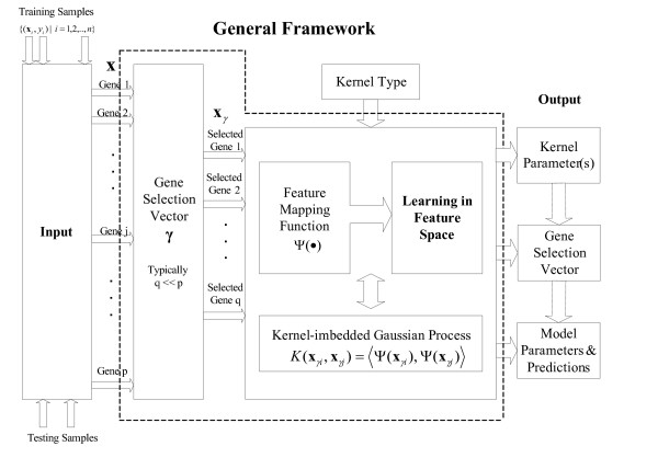
Results: A hierarchical statistical model named kernel-imbedded Gaussian process (KIGP) is developed under a unified Bayesian framework for binary disease classification problems using microarray gene expression data. In particular, based on a probit regression setting, an adaptive algorithm with a cascading structure is designed to find the appropriate kernel, to discover the potentially significant genes, and to make the optimal class prediction accordingly. A Gibbs sampler is built as the core of the algorithm to make Bayesian inferences. Simulation studies showed that, even without any knowledge of the underlying generative model, the KIGP performed very close to the theoretical Bayesian bound not only in the case with a linear Bayesian classifier but also in the case with a very non-linear Bayesian classifier. This sheds light on its broader usability to microarray data analysis problems, especially to those that linear methods work awkwardly. The KIGP was also applied to four published microarray datasets, and the results showed that the KIGP performed better than or at least as well as any of the referred state-of-the-art methods did in all of these cases.

Conclusion: Mathematically built on the kernel-induced feature space concept under a Bayesian framework, the KIGP method presented in this paper provides a unified machine learning approach to explore both the linear and the possibly non-linear underlying relationship between the target features of a given binary disease classification problem and the related explanatory gene expression data. More importantly, it incorporates the model parameter tuning into the framework. The model selection problem is addressed in the form of selecting a proper kernel type. The KIGP method also gives Bayesian probabilistic predictions for disease classification. These properties and features are beneficial to most real-world applications. The algorithm is naturally robust in numerical computation. The simulation studies and the published data studies demonstrated that the proposed KIGP performs satisfactorily and consistently.

Figure 1

Schematic plot for the general framework of the proposed KIGP method.

Figure 2

The results from applying the KIGP with an GK to one of the training sets of the simulated example 1, where (a) and (b) are for the linear case; (c) and (d) are for the non-liner case. (a) The estimated marginal posterior PDF of the width parameter of the GK (solid line) versus its prior PDF (dotted line). The mode of the posterior PDF is at around 1.61. (b) The local fdr with the GK(1.61) (with the standard normal as the density of NLF under null hypothesis); the horizontal dotted line represents the threshold of the fdr (0.05); the vertical dotted line shows the resulted cutoff value for NLF (3.83). (c) The estimated marginal posterior PDF of the width parameter of the GK (solid line) versus its prior PDF (dotted line). The mode of the posterior PDF is at around 0.81. (d) The local fdr with the GK(0.81) (with standard normal as the density of NLF under null hypothesis); the horizontal dotted line represents the threshold of the fdr (0.05); the vertical dotted line shows the resulted cutoff value for NLF (3.68).

Figure 3

The results from applying the KIGP to one of the training sets of the linear case in the simulated example 1, where (a) and (b) are for the simulation with an LK; (c) and (d) are for the one with an GK; (e) and (f) for the one with an PK. (a) The NLF plot of each gene for the simulation with an LK; with the cutoff value for NLF (dotted line), two genes were found significant (the circles mark the preset significant genes). (b) The contours of the posterior predictive probability of the class "1" for the simulation with an LK, where X-axis is for the value of the gene 23 and Y-axis represents the value of the gene 57; the numbers associated with contours are the probabilities; the asterisks denote the training samples from the class "1"; the circles demonstrate the training samples from the class "-1"; the dotted line shows the Bayesian classifier. For this set of training samples, the testing MR is 0.022 (the Bayesian bound for MR is 0.013). (c) Same as (a) except it is for the simulation with an GK. (d) Same as (b) except it is for the simulation with an GK. The testing MR is 0.028. (e) Same as (a) except it is for the simulation with an PK. (f) Same as (b) except it is for the simulation with an PK. The testing MR is 0.017.

Figure 4

The results from applying the KIGP to one of the training sets for the non-linear case in the simulated example 1, where (a) and (b) are for the simulation with an LK; (c) and (d) are for the simulation with an GK; (e) and (f) for the simulation with an PK. All the legends are same as those in Fig. 3. (a) The NLF plot of each gene for the simulation with an LK; with the cutoff value for NLF (dotted line), none of the true preset significant genes was found (2 false negatives). Three false positive genes were misclassified as significant. (b) The contours of the posterior predictive probability of the class "1" for the simulation with an LK (given the two true preset significant genes). For this set of training samples, the testing MR is 0.5 (the Bayesian bound is 0.055). (c) Same as (a) except it is for the simulation with an GK. (d) Same as (b) except it is for the simulation with an GK. The testing MR is 0.063. (e) Same as (a) except it is for the simulation with an PK. (f) Same as (b) except it is for the simulation with an PK. The testing MR is 0.060.

Figure 5

The results from applying the KIGP to one of the training sets of the simulated example 2, where (a) and (b) are for the simulation with an PK; (c) and (d) are for the simulation with an GK. (a) The estimated marginal posterior PMF of the degree parameter d. (b) The NLF plot of each gene for the simulation with the PK(2); the dots mark the prescribed significant genes. For this training set, all 10 preset significant genes and 1 false positive gene were found. (c) The estimated marginal posterior PDF of the width parameter r (solid line) versus its prior PDF (dotted line). The mode of the posterior PDF is at around 0.64. (d) The NLF plot for each gene for the simulation with the GK(0.64). The legends are same as those in (b). For this training set, all 10 preset significant genes were found with no false positive result.

Figure 6

The heat map of the gene expression levels of the 20 found significant genes for the acute leukemia dataset. The panel on the left (to the solid line) represents the training samples and that on the right shows the testing samples. The two dotted lines are used to separate the two classes (ALL and AML).

Figure 8

The NLF plots for all 4 real data studies with found kernels. The legends are same for all four plots. (a) The NLF plot of each gene with the LK for the leukemia dataset and the dots mark the 20 found significant genes, the details of which are listed in Table 3. (b) The NLF plot of each gene with the PK(1) for the SRBCT dataset and the details of the 15 found significant genes are listed in Table 5. (c) The NLF plot of each gene with the GK(3.19) for the breast cancer dataset and the details of the 9 found significant genes are listed in Table 7. (d) The NLF plot of each gene with the GK(2.38) for the colon dataset and the details of the 8 found significant genes are listed in Table 9.

Figure 9

The estimated marginal posterior PDF of the width parameter of an GK for each real data study case (dotted lines present the prior PDF). (a) For the leukemia dataset, the mode of the posterior PDF is at around 2.79. (b) For the SRBCT dataset, the mode of the posterior PDF is at around 2.36. (c) For the breast cancer dataset, the mode of the posterior PDF is at around 3.19. (We also noticed that there was a local peak on the left, which was at around 0.56). (d) For the colon dataset, the mode of the posterior PDF is at around 2.38.

Figure 7

The heat map of the gene expression levels of the 15 found significant genes for the SRBCT dataset. All the legends are same as those in Fig. 6 except that the two classes are EWS and NB.

References

1. Golub TR, Slonim D, Tamayo P, Huard C, Gaasenbeek M, Mesirov J, Coller H, Loh M, Downing J, Caligiuri M, Bloomfield C, Lender E. Molecular classification of cancer: class discovery and class prediction by gene expression monitoring. Science. 1999;286:531–537. doi: 10.1126/science.286.5439.531. - DOI - PubMed
1. Golub TR. Genome-Wide Views of Cancer. N Engl J Med. 2001;344:601–602. doi: 10.1056/NEJM200102223440809. - DOI - PubMed
1. Ramaswamy S, Golub TR. DNA Microarrays in Clinical Oncology. Journal of Clinical Oncology. 2002;20:1932–1941. - PubMed
1. Tamayo P, Ramaswamy S. In: "Cancer Genomics and Molecular Pattern Recognition" in Expressing profiling of human tumors: diagnostic and research applications. Marc Ladanyi, William Gerald, editor. Human Press; 2003.
1. Mallows CL. Some comments on Cp. Technometrics. 1973;15:661–676. doi: 10.2307/1267380. - DOI
Publication types
MeSH terms
LinkOut - more resources