A maximum-likelihood method for the estimation of pairwise relatedness in structured populations

Abstract

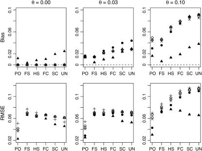
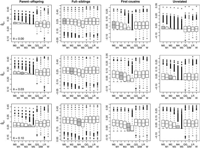
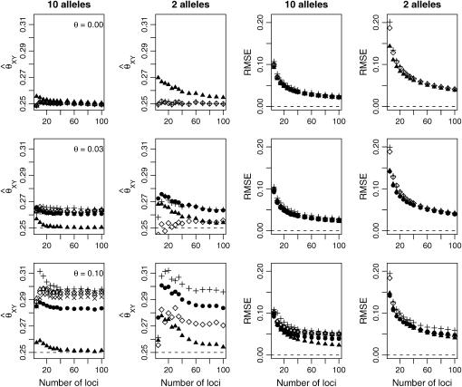
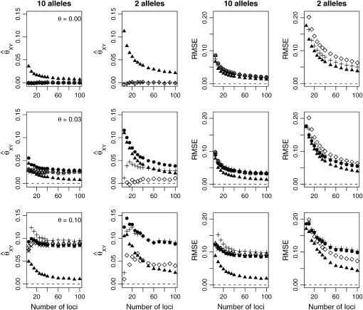
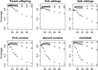
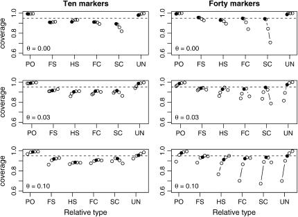
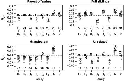
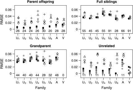
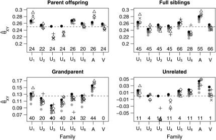
A maximum-likelihood estimator for pairwise relatedness is presented for the situation in which the individuals under consideration come from a large outbred subpopulation of the population for which allele frequencies are known. We demonstrate via simulations that a variety of commonly used estimators that do not take this kind of misspecification of allele frequencies into account will systematically overestimate the degree of relatedness between two individuals from a subpopulation. A maximum-likelihood estimator that includes F(ST) as a parameter is introduced with the goal of producing the relatedness estimates that would have been obtained if the subpopulation allele frequencies had been known. This estimator is shown to work quite well, even when the value of F(ST) is misspecified. Bootstrap confidence intervals are also examined and shown to exhibit close to nominal coverage when F(ST) is correctly specified.

Figure 1.—

Jacquard's identity-by-descent modes. Each group of four dots represents an IBD mode between two individuals. The top pair of dots represents the two alleles in individual 1 and the bottom pair of dots represents the two alleles in individual 2. Lines connect alleles that are IBD.

Figure 2.—

Average behavior in subpopulations of a population in which allele frequencies follow a triangle distribution. Here we show the average bias and RMSE based on 1000 relative pairs of each type drawn from each of 4000 simulated subpopulations. The symbols are as follows: •, rMLE; ▴, fMLE; ▵, Queller–Goodnight; +, Lynch–Ritland; x, similarity index; ⋄, Wang.

Figure 3.—

Box plots showing the distribution of the estimators on a single subpopulation. We simulated 5000 relative pairs of each type for each of three values of θ. The top row of plots shows the results when the relative pair comes from a subpopulation with θ = 0.0, whereas the middle and bottom rows of plots show results when the simulations were run with θ = 0.03 and θ = 0.10, respectively. We estimated the relatedness of the individuals using the four moment estimators as well as the maximum-likelihood estimators assuming various values of θ. The symbols for the maximum-likelihood estimators are: M0, θ = 0.00; M1, θ = 0.01; M2, θ = 0.03; M3, θ = 0.05; M4, θ = 0.10; M5, θ = 0.15. The MLE that assumes the correct value of θ for the subpopulation is shaded. The box plots shown contain boxes that extend from the first to the third quartiles of the relatedness estimates, with a line through the box indicating the median. Whiskers extend from the boxes to the most extreme data point that is within 1.5 times the interquartile range from the box.

Figure 4.—

Full siblings. Here, we have generated 10,000 full-sibling pairs from a single subpopulation and examined the effect of the number of loci and number of possible alleles on relationship estimation. The symbols for the various estimators are as given in Figure 2.

Figure 5.—

Unrelateds. Here, we have generated 10,000 pairs of unrelated individuals from a single subpopulation and examined the effect of the number of loci and number of possible alleles on relationship estimation. The symbols for the various estimators are as given in Figure 2.

Figure 6.—

Coverage probabilities based on the reduced-model MLE when relative pairs were generated from a subpopulation with θ = 0.0 (○), θ = 0.03 (▵), and θ = 0.10 (+).

Figure 7.—

Effects of parameter misspecification on confidence interval coverage. Each plot shows the empirical coverage probabilities for bootstrap confidence intervals based on a fixed number of markers (10 or 40) and a set degree of population structure (θ = 0.00, 0.03, 0.10). Within each plot, for each type of relative pair is the coverage of 95% confidence intervals based on 1000 pairs of individuals, where the analysis was performed under various assumed values of θ. When the true value of θ was 0.00, we analyzed each pair of individuals under the assumed values of (left to right) θ = 0.00, 0.01, 0.03, and 0.05. When the true value of θ was 0.03, we analyzed the data under assumed values of θ = 0.00, 0.01, 0.03, 0.05, and 0.08. Finally, when θ was 0.10, we performed analyses under assumed values of θ = 0.05, 0.08, 0.10, 0.12, and 0.15. In all cases, the results when the true value of θ was assumed are represented by a solid circle. All other values of θ are indicated by open circles.

Figure 8.—

Mean estimates for the CEPH data set, based on the first set of 49 loci. The families are denoted as follows: U₁, …, U₆ refer to Utah families 1331, 1332, 1347, 1362, 1413, and 1416; A refers to the Old Order Amish family 884; V refers to the Venezuelan family 102. For each family, we have plotted the mean estimates in two columns: The left column has the MLE estimates calculated with θ = 0.0, 0.01, 0.02, 0.03, 0.05. All MLEs are indicated by solid circles, with darker shaded circles indicating lower values of θ. The right column has the other estimators with symbols as follows: ▵, Queller–Goodnight; +, Lynch–Ritland; x, similarity index; ⋄, Wang. Above the horizontal axis are values indicating the number of relative pairs evaluated in each family.

Figure 9.—

Root mean-square error for the CEPH data set, based on the first set of 40 loci. The symbols for this plot are the same as those in Figure 8.

Figure 10.—

Mean estimates for the CEPH reference families, as generated by a second set of markers. The symbols in this plot are the same as those in Figure 8.

References

1. Ayres, K. L., 2000. Relatedness testing in subdivided populations. Forensic Sci. Int. 114: 107–115. - PubMed
1. Balding, D. J., and R. A. Nichols, 1994. DNA profile match probability calculation: how to allow for population stratification, relatedness, database selection and single bands. Forensic Sci. Int. 64: 125–140. - PubMed
1. Balding, D. J., and R. A. Nichols, 1997. Significant genetic correlations among Caucasians at forensic DNA loci. Heredity 78: 583–589. - PubMed
1. Broman, K. W., and J. L. Weber, 1999. Long homozygous chromosomal segments in reference families from the Centre d'Ètude du Polymorphisme Humain. Am. J. Hum. Genet. 65: 1493–1500. - PMC - PubMed
1. Budowle, B., and K. L. Monson, 1994. Greater differences in forensic DNA profile frequencies estimated from racial groups than from ethnic subgroups. Clin. Chim. Acta 228: 3–18. - PubMed
Publication types