Scale-invariant memory representations emerge from moiré interference between grid fields that produce theta oscillations: a computational model

Abstract

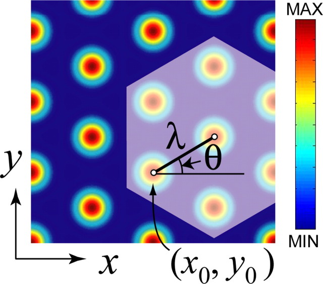
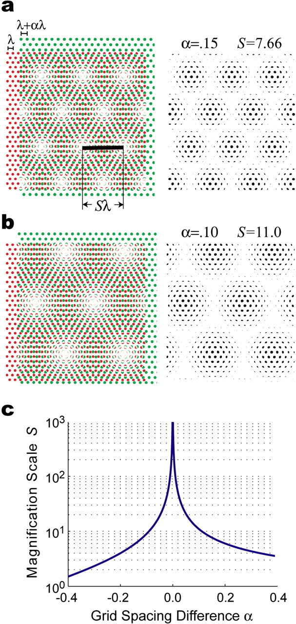
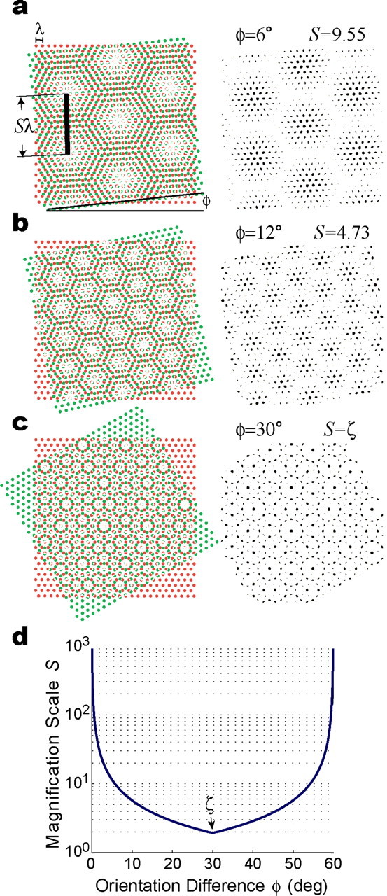
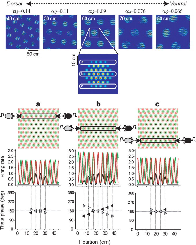
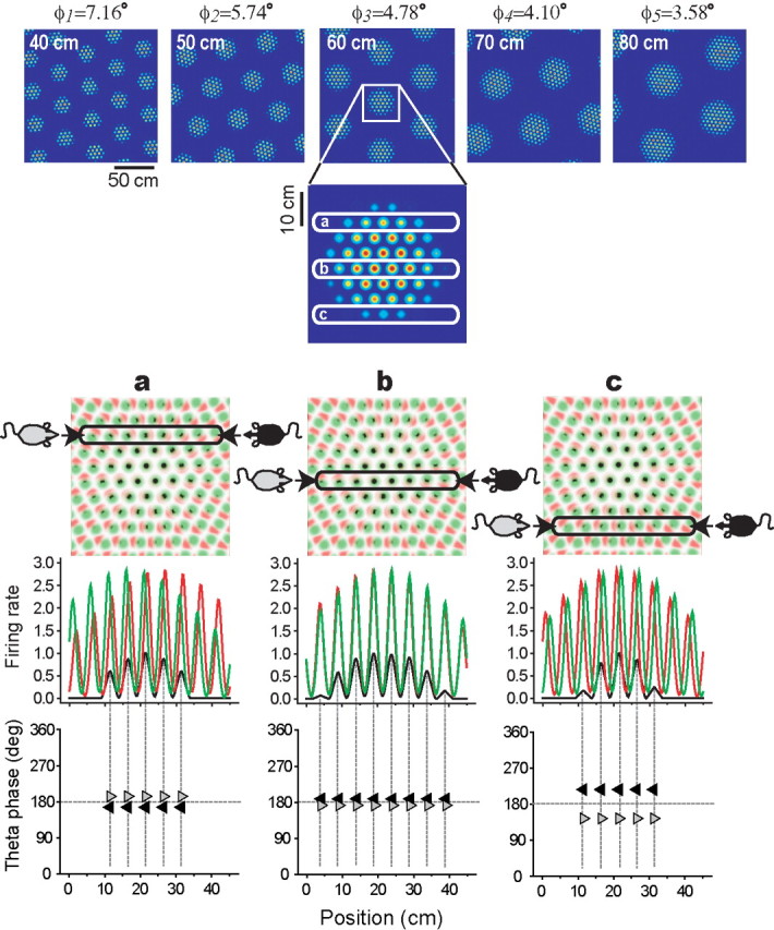
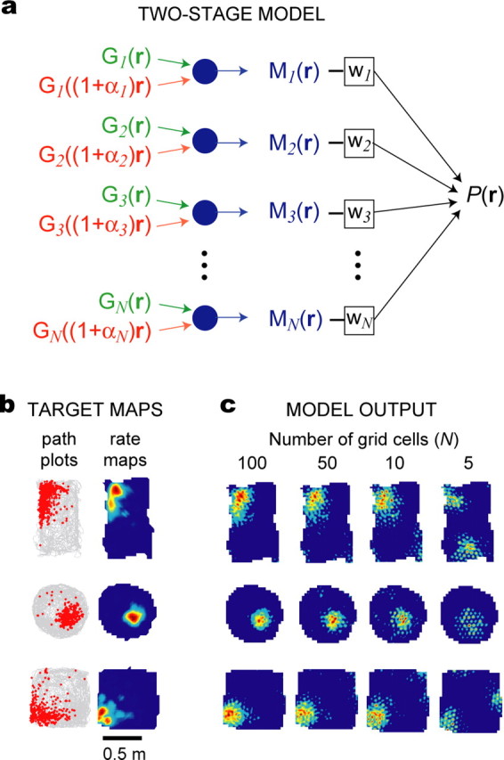
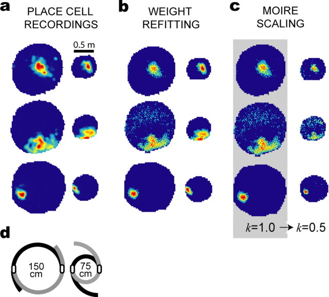
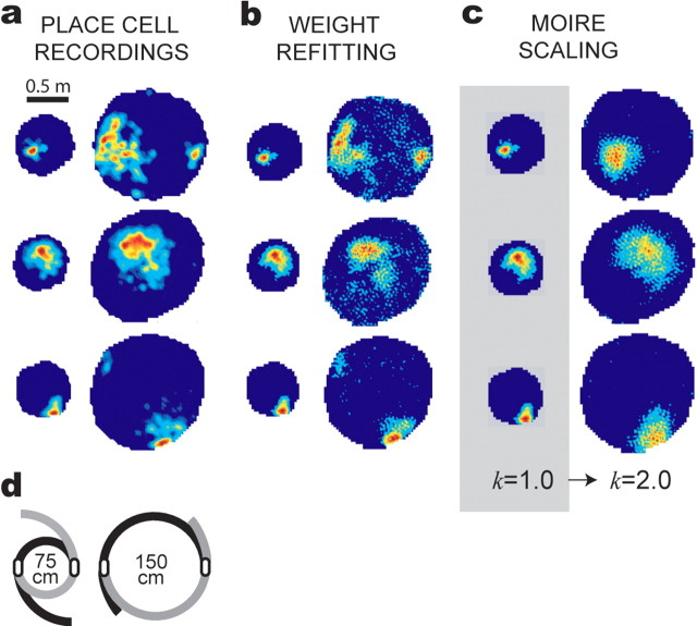
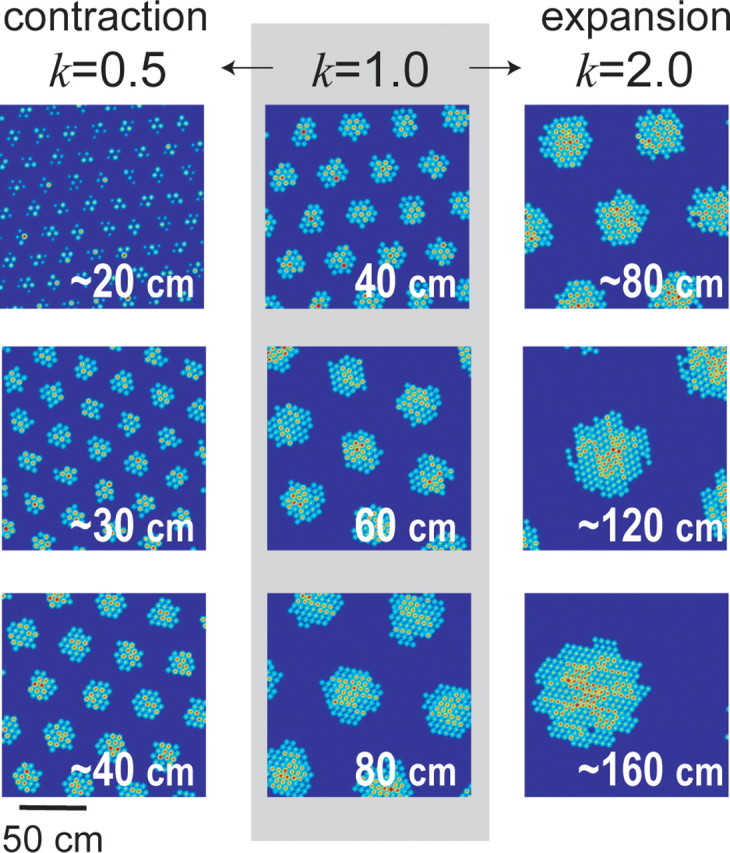
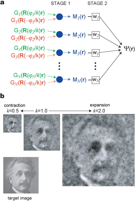
The dorsomedial entorhinal cortex (dMEC) of the rat brain contains a remarkable population of spatially tuned neurons called grid cells (Hafting et al., 2005). Each grid cell fires selectively at multiple spatial locations, which are geometrically arranged to form a hexagonal lattice that tiles the surface of the rat's environment. Here, we show that grid fields can combine with one another to form moiré interference patterns, referred to as "moiré grids," that replicate the hexagonal lattice over an infinite range of spatial scales. We propose that dMEC grids are actually moiré grids formed by interference between much smaller "theta grids," which are hypothesized to be the primary source of movement-related theta rhythm in the rat brain. The formation of moiré grids from theta grids obeys two scaling laws, referred to as the length and rotational scaling rules. The length scaling rule appears to account for firing properties of grid cells in layer II of dMEC, whereas the rotational scaling rule can better explain properties of layer III grid cells. Moiré grids built from theta grids can be combined to form yet larger grids and can also be used as basis functions to construct memory representations of spatial locations (place cells) or visual images. Memory representations built from moiré grids are automatically endowed with size invariance by the scaling properties of the moiré grids. We therefore propose that moiré interference between grid fields may constitute an important principle of neural computation underlying the construction of scale-invariant memory representations.

Figure 1.

Simulated grid fields. Example of a simulated grid cell firing field generated by the cosine grating model that was used in our simulations. Hot colors correspond to grid vertices at which the firing rate of the cell is high, and cold colors indicate regions of low firing (the firing rate scale is arbitrary). The hexagonal grid pattern can be characterized by three parameters: grid spacing (λ), angular orientation (θ), and spatial phase [c = (x₀, y₀)].

Figure 2.

The length scaling rule. a, Two basis grids with identical angular orientation but different vertex spacings, λ (red) and λ + αλ (green), intersect to form a moiré grid shown in black to the right of the basis grids. The vertex spacing of the moiré grid is Sλ, where S is a scaling factor that depends on α. In this example, α = 0.15 and S = 7.66. b, Another example of a moiré grid formed by the length scaling rule, with α = 0.10 and S = 11.0. c, The scaling factor S depends on α, which determines the difference between the spacings of the two basis grids (see Eq. 2).

Figure 3.

The rotational scaling rule. a, Two basis grids with identical vertex spacing λ and orientations which differ by angle φ intersect to form a moiré grid shown in black to the right of the basis grids. The vertex spacing of the moiré grid is Sλ, where S is a scaling factor that depends on φ. In this example, φ = 6° and S = 9.55. b, Another example of a moiré grid formed by the rotational scaling rule, with φ = 12° and S = 4.73. c, When φ = 30°, the scaling factor becomes irrational (S = ζ), and the moiré grid becomes an aperiodic tessellation of the plane. d, The scaling factor S depends on the separation angle, φ, between the orientations of the basis grids (see Eq. 3); note the irrational singular point at φ = 30°, at which the scale of magnification is S = ζ.

Figure 4.

Simulations of layer II grid cells. Top row, Five moiré grid fields, M_i(r), produced by the length scaling rule (Eq. 2); the spacing difference (α_i) between theta grids is shown above each plot, and the vertex spacing (S_iλ) of each moiré grid is shown at the top left corner of each plot (the hypothetical gradation of α_i along the dorsoventral axis of dMEC runs from left to right). Second row, A magnified inset of one moiré grid vertex and three different horizontal cross sections (a, b, and c) through the vertex. Third row, Magnified insets of the theta grids, with G_i(r) plotted in red, G_i((1 + α_i)r) plotted in green, and M_i(r) plotted in black. Fourth row, Simulated firing rates (y-axis) of the moiré grid cell (black) and theta grids (red and green) along three horizontal cross sections (columns a, b, and c). Fifth row, The phase of theta rhythm at which M_i(r) peaks on each cycle, with left-to-right traversals shown by gray arrows and right-to-left traversals shown by black arrows; the slopes of these plots show that phase precession occurs as the rat traverses the vertex in either direction (theta EEG is assumed to correspond to the green grid; see Results, Simulating layer II grid cells by the length scaling rule).

Figure 5.

Simulations of layer III grid cells. Top row, Five moiré grid fields, M_i(r), produced by the rotational scaling rule (Eq. 3); the separation angle (φ_i) between theta grids is shown above each plot, and the vertex spacing (S_iλ) of each moiré grid is shown at the top left corner of each plot. Second row, A magnified inset of one moiré grid vertex, with three different horizontal cross sections (a, b, and c) through the vertex. Third row, Magnified insets of the theta grids, with G_i(R(+ϕ_i)r) plotted in red, G_i(R(−ϕ_i)r) plotted in green, and M_i(r) plotted in black. Fourth row, Simulated firing rates (y-axis) of the moiré grid cell (black) and theta grids (red and green) along three horizontal cross sections (columns a, b, and c). Fifth row, The phase of theta rhythm at which M_i(r) peaks on each theta cycle for left-to-right traversals (gray arrows) and right-to-left traversals (black arrows). Lateral phase shifting can be seen by comparing across columns a, b, and c. In column b, the rat passes slightly below the center of the vertex, so M_i(r) fires at a slight phase shift from the middle of the theta cycle; in column c, the rat passes farther below the center of the vertex, so M_i(r) fires at a large phase shift from the middle of the theta cycle; in column a, the rat passes above the center of the vertex (farther from the center than in b but not as far as in c), so M_i(r) fires at a moderate phase shift from the middle of the theta cycle (note that in a, the direction of the phase shift is opposite from b and c, because the rat is passing above the vertex center rather than below it). Theta EEG is assumed to correspond to the green grid as in Figure 4.

Figure 6.

Building place cells from grid cells. a, Diagram of the two-stage model of place cells. b, Path plots (left) and firing rate maps (right) for three real place cells that were recorded in rectangular, circular, and square environments. c, Simulated firing rate maps produced by the two-stage model (see Eq. 15) with different numbers of grid cells in the basis set (N = 100, 50, 10, or 5).

Figure 7.

Place field contractions in the yin–yang maze. The yin–yang maze was contracted from the large (150 cm) to the small (75 cm) configuration during the recording session. a, Firing rate maps are shown for three different place cells recorded before and after maze contraction. b, Simulated firing rate maps constructed from a basis set of 200 grid cells, using different weight vectors (w^S and w^L) for the small and large rate maps. c, Simulated firing rate maps produced by the moiré model (200 grid cells); coefficients were fit to the large (precontraction) firing rate map (gray background), and the small map was then derived by reducing k from 1.0 to 0.5 without changing the coefficients. d, Overhead view shows how the maze was contracted during the recording session.

Figure 8.

Place field expansions in the yin–yang maze. The yin–yang maze was expanded from the small (75 cm) to the large (150 cm) configuration during the recording session. a, Firing rate maps are shown for three different place cells recorded before and after maze expansion. b, Simulated firing rate maps constructed from a basis set of 200 grid cells, using different weight vectors (w^S and w^L) for the small and large rate maps. c, Simulated firing rate maps produced by the moiré model (200 grid cells); coefficients were fit to the small (preexpansion) firing rate map (gray background), and the large map was then derived by increasing k from 1.0 to 2.0 without changing the coefficients. d, Overhead view shows how the maze was expanded during the recording session.

Figure 9.

Grid field rescaling. Three moiré grid fields (middle column, gray background) were simulated by the length scaling rule with the scaling parameter set to k = 1 (Eq. 17). When the scaling parameter was reduced to k = 0.5, grids rescaled by approximately halving their vertex spacings (left column). When the scaling parameter was increased to k = 2.0, grids rescaled by approximately doubling their vertex spacings (right column). The vertex spacing of the grid field is shown in the top left corner of each plot; rescaling is approximate rather than exact as explained in Appendix B.

Figure 10.

Scale-invariant representation of a visual image by moiré grids. a, Two-stage model for constructing image representations. b, The target image was a 272 × 272 pixel grayscale image (bottom left). Weighting coefficients for a basis set of 1500 grid fields were fit to the target image with k = 1.0. Then, a half-sized image was produced by setting k = 0.5, and a double-sized image was produced by setting k = 2.0. In these simulations, moiré grids were constructed using the rotational scaling rule, and the k parameter modulated the angle between the sibling grid pair that formed each moiré grid.

References

1. Amidror I. The theory of the moiré phenomenon. Kluwer Academic; 2000.
1. Barry C, Lever C, Hayman R, Hartley T, Burton S, O'Keefe J, Jeffery K, Burgess N. The boundary vector cell model of place cell firing and spatial memory. Rev Neurosci. 2006;17:71–97. - PMC - PubMed
1. Biederman I, Cooper EE. Size invariance in visual object priming. J Exp Psychol Hum Percept Perform. 1992;18:121–133.
1. Brown MW, Aggleton JP. Recognition memory: what are the roles of the perirhinal cortex and hippocampus? Nat Rev Neurosci. 2001;2:51–61. - PubMed
1. Burgess N, Barry C, Jefferies KJ, O'Keefe J. A grid and place cell model of path integration utilizing phase precession versus theta. 1st Annual Conference on Computational Cognitive Neuroscience; Washington, DC. 2005.
Publication types