Global patterns and determinants of vascular plant diversity

Abstract

Plants, with an estimated 300,000 species, provide crucial primary production and ecosystem structure. To date, our quantitative understanding of diversity gradients of megadiverse clades such as plants has been hampered by the paucity of distribution data. Here, we investigate the global-scale species-richness pattern of vascular plants and examine its environmental and potential historical determinants. Across 1,032 geographic regions worldwide, potential evapotranspiration, the number of wet days per year, and measurements of topographical and habitat heterogeneity emerge as core predictors of species richness. After accounting for environmental effects, the residual differences across the major floristic kingdoms are minor, with the exception of the uniquely diverse Cape Region, highlighting the important role of historical contingencies. Notably, the South African Cape region contains more than twice as many species as expected by the global environmental model, confirming its uniquely evolved flora. A combined multipredictor model explains approximately 70% of the global variation in species richness and fully accounts for the enigmatic latitudinal gradient in species richness. The models illustrate the geographic interplay of different environmental predictors of species richness. Our findings highlight that different hypotheses about the causes of diversity gradients are not mutually exclusive, but likely act synergistically with water-energy dynamics playing a dominant role. The presented geostatistical approach is likely to prove instrumental for identifying richness patterns of the many other taxa without single-species distribution data that still escape our understanding.

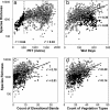
Fig. 1.

Relationship between environmental predictors and species richness of vascular plants in low- and high-energy regions. Species richness is standardized to 10,000 km². (a) The effect of PET [millimeters per year (mm/a)] on species richness. A close association is observed in regions with <505 mm/a PET (filled circles), whereas in regions with higher energy input (open circles) the relationship is not significant (breakpoint confirmed by split-line regression). (b–d) Also shown are relationships for wet days (b), topographical complexity measured as the number of elevational bands (c), and heterogeneity measured in number of vegetation types per region (d).

Fig. 2.

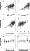
Partial residuals plots for all variables included in the combined model of global plant richness (compare Table 2). These plots show the effects of a given variable when all others in the model are statistically controlled for. (a–e) Hatched lines partial fits. (e and f) Boxes indicate second and third quartiles, black notches denote 95% confidence intervals, and whiskers indicate 10th and 90th percentiles. NEA, Nearctic; PAA, Palaearctic; NET, Neotropic; PAT, Paleotropic; CAP, Cape; AUS, Australis. Note high partial residuals of the Cape floristic kingdom after controlled-for environmental differences (∗∗∗, significant at P < 0.001; Tukey post hoc test). Specifically, a partial residual plot is a plot of r_i + b_k × i_k vs. x_ik, where r_i is the ordinary residual for the ith observation, x_ik is the ith observation of the kth predictor, and b_k is the regression coefficient estimate for the kth predictor.

Fig. 3.

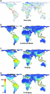
Global patterns of vascular plant species richness. (a) The geographic distribution of the richness data of vascular plants for the 1,032 geographic regions analyzed in this study (each dot presents the mass centroid of a geographic entity; note that regions differ in size and that species counts have not been standardized). (b–d) The species-richness maps show area-standardized predictions of three different global models across an equal area grid (≈12,100 km², ≈1° latitude × 1° longitude near the equator) based on the combined multipredictor model (b), ordinary kriging of species richness (where species richness is interpolated purely as a function of spatial autocorrelation in the response variable) (c), and ordinary cokriging (which incorporates both the spatial autocorrelation in species richness and the combined model as an underlying trend) (d).

References

1. Schall JJ, Pianka ER. Science. 1978;201:679–686. - PubMed
1. Wright DH. Oikos. 1983;41:496–506.
1. Rohde K. Oikos. 1992;65:514–527.
1. Hawkins BA, Field R, Cornell HV, Currie DJ, Guégan J-F, Kaufman DM, Kerr JT, Mittelbach GG, Oberdorff T, O'Brien EM, et al. Ecology. 2003;84:3105–3117.
1. Currie DJ, Mittelbach G, Cornell HV, Field R, Guégan J, Hawkins BA, Kaufman DM, Kerr JT, Oberdorff T, O'Brien EM, Turner JRG. Ecol Lett. 2004;7:1121–1134.
Publication types
LinkOut - more resources