Estimating the number of ancestral lineages using a maximum-likelihood method based on rejection sampling

Abstract

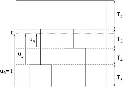
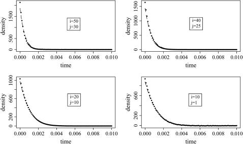
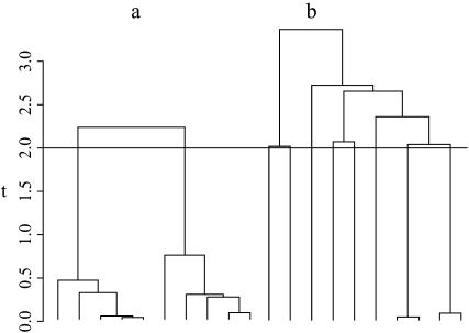
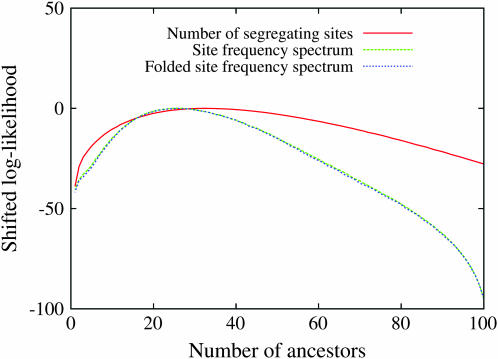
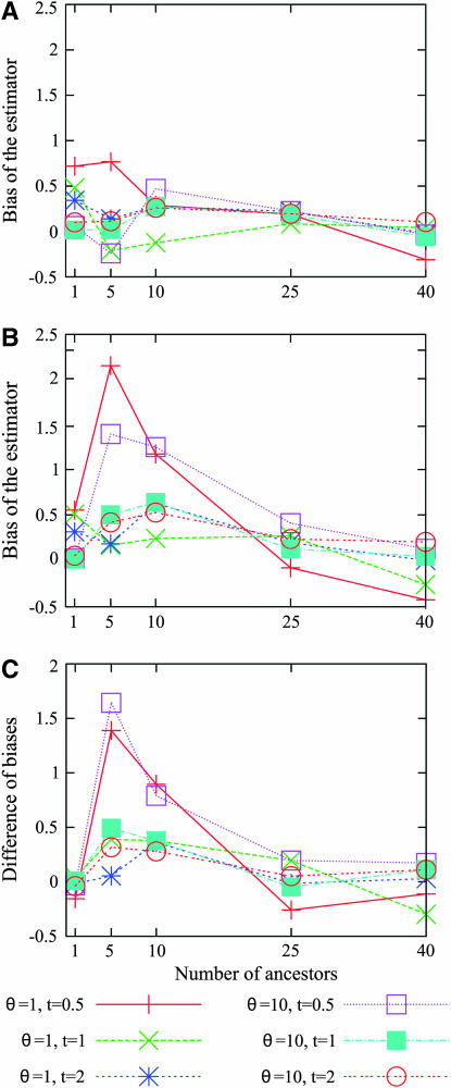
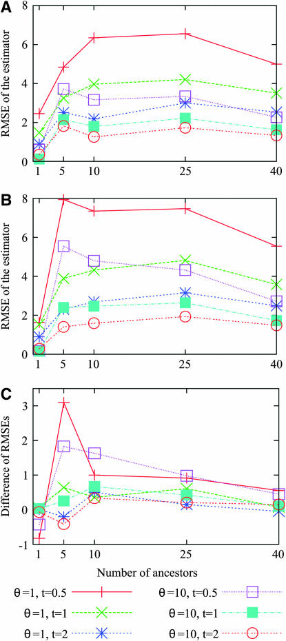
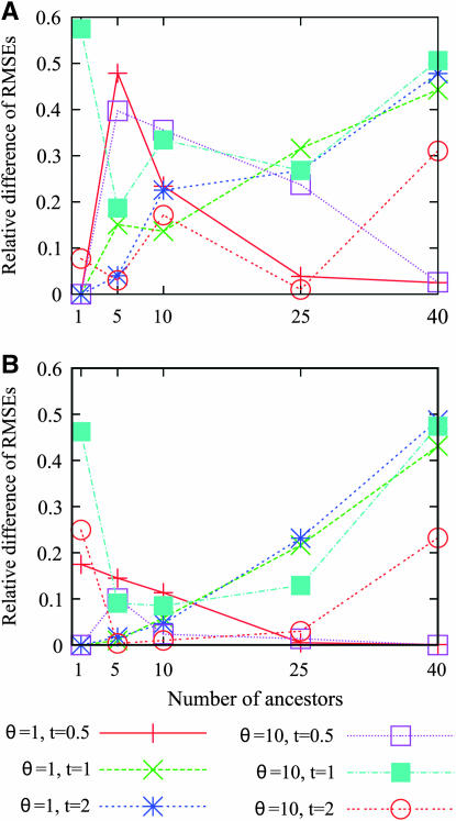
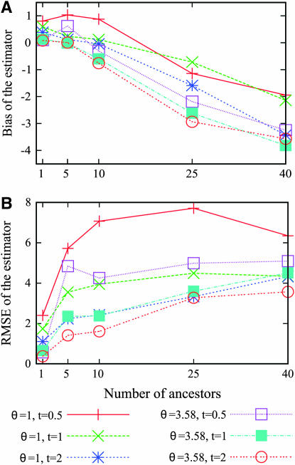
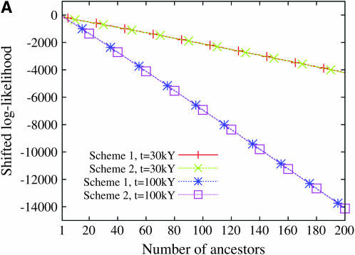
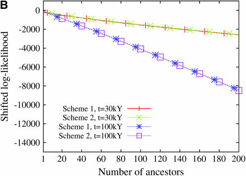
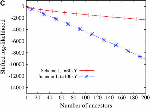
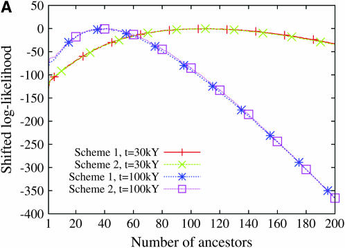
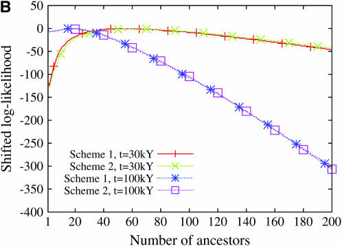
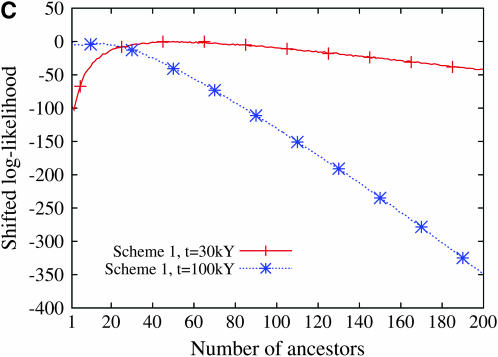
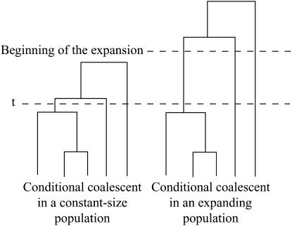
Estimating the number of ancestral lineages of a sample of DNA sequences at time t in the past can be viewed as a variation on the problem of estimating the time to the most recent common ancestor. To estimate the number of ancestral lineages, we develop a maximum-likelihood approach that takes advantage of a prior model of population demography, in addition to the molecular data summarized by the pattern of polymorphic sites. The method relies on a rejection sampling algorithm that is introduced for simulating conditional coalescent trees given a fixed number of ancestral lineages at time t. Computer simulations show that the number of ancestral lineages can be estimated accurately, provided that the number of mutations that occurred since time t is sufficiently large. The method is applied to 986 present-day human sequences located in hypervariable region 1 of the mitochondrion to estimate the number of ancestral lineages of modern humans at the time of potential admixture with the Neanderthal population. Our estimates support a view that the proportion of the modern population consisting of Neanderthal contributions must be relatively small, less than approximately 5%, if the admixture happened as recently as 30,000 years ago.

Figure 1.—

A coalescent tree with n = 5 sequences conditioned on having j = 3 lineages at time t. The T_i's correspond to the intercoalescence times and u_i corresponds to the time elapsed between the (n − i)th coalescence event and time t.

Figure 2.—

For different values of i and j, the exact (Equation 4) and approximate p.d.f. (Equation 6) of the intercoalescence time T_i given that A_n(t) = j and . The dashed lines correspond to the approximate p.d.f. and the points correspond to the exact p.d.f. The time elapsed between and t is fixed at u_i+1 = 0.01.

Figure 3.—

Two coalescent trees with n = 10 individuals conditional on having, at time t = 2, (a) j = 2 lineages or (b) j = 8 lineages. Both trees were simulated using Algorithm 2.

Figure 4.—

The profile of the log-likelihood of the number of ancestors estimated from a simulated data set summarized in each of three ways. The number of sequences was set at n = 100 and the number of ancestors 1 coalescent time unit before the present was set at 25. The mutation rate was fixed at θ = 5. The log-likelihood functions have been shifted so that their maximum values are 0.

Figure 5.—

The bias of the estimator, . At each of several values for the number of ancestors at time t, the bias was estimated using 1000 simulated genetic data sets with a sample size of n = 50. (A) Bias for the estimator based on the site frequency spectrum. (B) Bias for the estimator based on the folded site frequency spectrum. (C) Bias in B minus bias in A.

Figure 6.—

The root mean square error (RMSE) of the estimator, . At each of several values for the number of ancestors at time t, the RMSE was estimated using 1000 simulated genetic data sets with a sample size of n = 50. (A) RMSE for the estimator based on the site frequency spectrum. (B) RMSE for the estimator based on the folded site frequency spectrum. (C) RMSE in B minus RMSE in A.

Figure 7.—

The relative difference between the RMSE of the estimator computed from the number of segregating sites and the RMSE of the estimator computed from the (A) site frequency spectrum or the (B) folded site frequency spectrum [the relative difference between two variables A and B is defined by (A − B)/A]. At each of several values for the number of ancestors at time t, the RMSEs were estimated using 1000 simulated genetic data sets with a sample size of n = 50.

Figure 8.—

The (A) bias and the (B) RMSE of the estimator when the genetic data are simulated according to a finite-sites model. At each of several values for the number of ancestors at time t, the RMSEs were estimated using 1000 simulated genetic data sets with a sample size of n = 50.

Figure 9.—

The log-likelihood of the number of ancestral lineages of 986 human HV1 sequences, 30,000 years ago and 100,000 years ago. The likelihood was computed using a mutation rate of 5 × 10⁻⁵/site/generation. Scheme 1 and scheme 2 correspond to the two binning schemes (see Table 2). The log-likelihood functions have been shifted so that their maximum values are 0. (A) Constant population size, (B) one stage of population expansion, (C) two stages of population expansion.

Figure 9.—

The log-likelihood of the number of ancestral lineages of 986 human HV1 sequences, 30,000 years ago and 100,000 years ago. The likelihood was computed using a mutation rate of 5 × 10⁻⁵/site/generation. Scheme 1 and scheme 2 correspond to the two binning schemes (see Table 2). The log-likelihood functions have been shifted so that their maximum values are 0. (A) Constant population size, (B) one stage of population expansion, (C) two stages of population expansion.

Figure 9.—

The log-likelihood of the number of ancestral lineages of 986 human HV1 sequences, 30,000 years ago and 100,000 years ago. The likelihood was computed using a mutation rate of 5 × 10⁻⁵/site/generation. Scheme 1 and scheme 2 correspond to the two binning schemes (see Table 2). The log-likelihood functions have been shifted so that their maximum values are 0. (A) Constant population size, (B) one stage of population expansion, (C) two stages of population expansion.

Figure 10.—

The log-likelihood of the number of ancestral lineages of 986 human HV1 sequences 30,000 years and 100,000 years ago. The likelihood was computed using a mutation rate of 2.5 × 10⁻⁶/site/generation. Scheme 1 and scheme 2 correspond to the two binning schemes (see Table 2). The log-likelihood functions have been shifted so that their maximum values are 0. (A) Constant population size, (B) one stage of population expansion, (C) two stages of population expansion.

Figure 10.—

The log-likelihood of the number of ancestral lineages of 986 human HV1 sequences 30,000 years and 100,000 years ago. The likelihood was computed using a mutation rate of 2.5 × 10⁻⁶/site/generation. Scheme 1 and scheme 2 correspond to the two binning schemes (see Table 2). The log-likelihood functions have been shifted so that their maximum values are 0. (A) Constant population size, (B) one stage of population expansion, (C) two stages of population expansion.

Figure 10.—

The log-likelihood of the number of ancestral lineages of 986 human HV1 sequences 30,000 years and 100,000 years ago. The likelihood was computed using a mutation rate of 2.5 × 10⁻⁶/site/generation. Scheme 1 and scheme 2 correspond to the two binning schemes (see Table 2). The log-likelihood functions have been shifted so that their maximum values are 0. (A) Constant population size, (B) one stage of population expansion, (C) two stages of population expansion.

Figure 11.—

A genealogical tree of n = 5 individuals conditioned on having three lineages at time t, in a population of constant size and in an expanding population for which the beginning of the expansion is more ancient than t. The initial population size in the expanding population is the same as the present-day population size in the constant-population-size model. Because the coalescent tree in the expanding population is likely to have a longer total length, the number of mutations that occur along the genealogy from the expanding population is likely to be larger. Thus, the same number of ancestral lineages at time t will produce a larger genetic diversity in the expanding population. When analyzing the same amount of genetic diversity, this explains why the maximum-likelihood estimates of the number of ancestral lineages are smaller when assuming an expanding population rather than a constant-size population.

References

1. Bandelt, H.-J., L. Quintana-Murci, A. Salas and V. Macaulay, 2002. The fingerprint of phantom mutations in mitochondrial DNA data. Am. J. Hum. Genet. 71: 1150–1160. - PMC - PubMed
1. Beaumont, M. A., W. Zhang and D. J. Balding, 2002. Approximate Bayesian computation in population genetics. Genetics 162: 2025–2035. - PMC - PubMed
1. Bignami, A., and A. De Matteis, 1971. A note on sampling from combinations of distributions. IMA J. Appl. Math. 8: 80–81.
1. Biraben, J.-N., 1979. Essai sur l'évolution du nombre des hommes. Population 1: 13–25.
1. Blum, M. G. B., and O. François, 2005. On statistical tests of phylogenetic tree imbalance: the Sackin and other indices revisited. Math. Biosci. 195: 141–153. - PubMed
Publication types