Semiparametric bayesian inference for multilevel repeated measurement data

Abstract

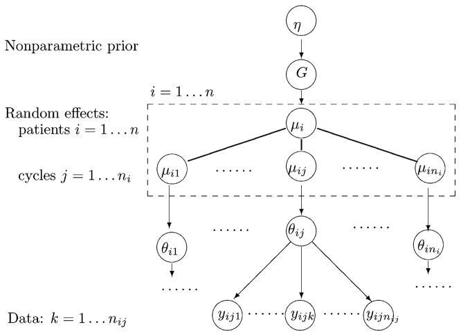
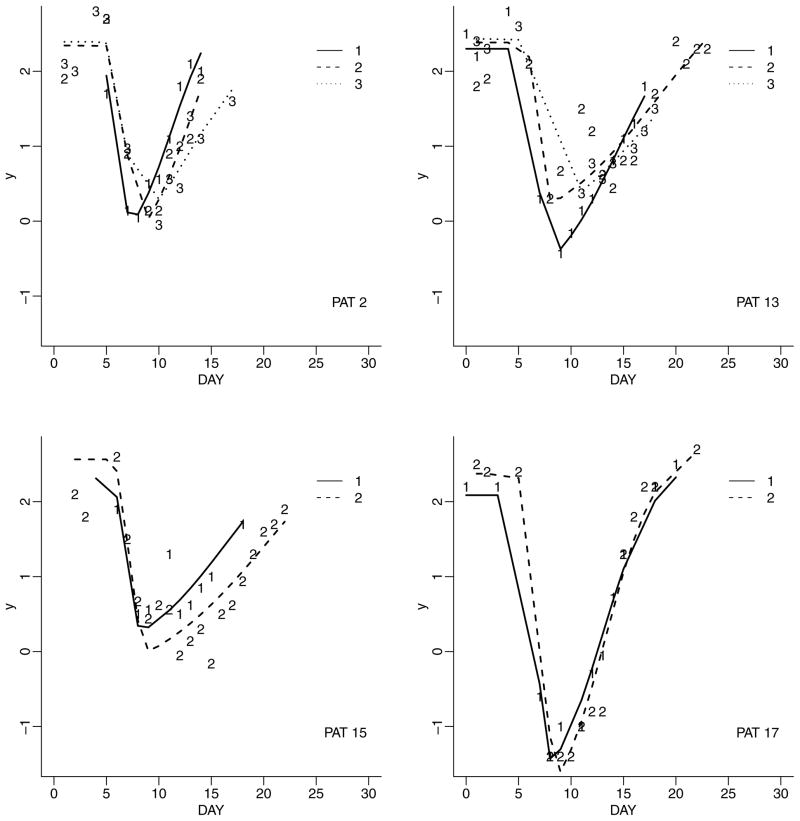
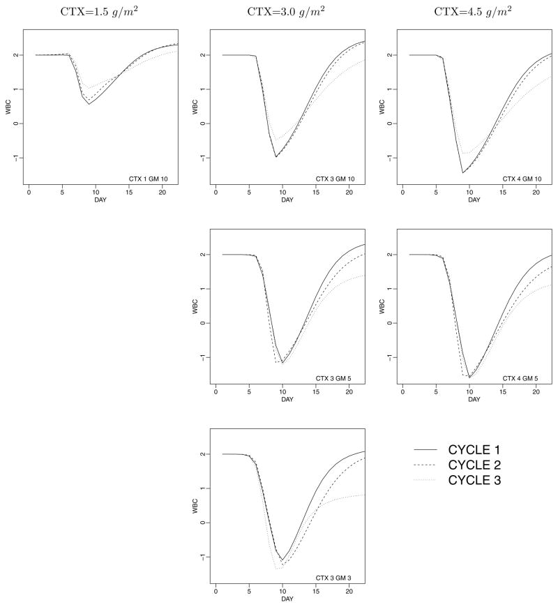
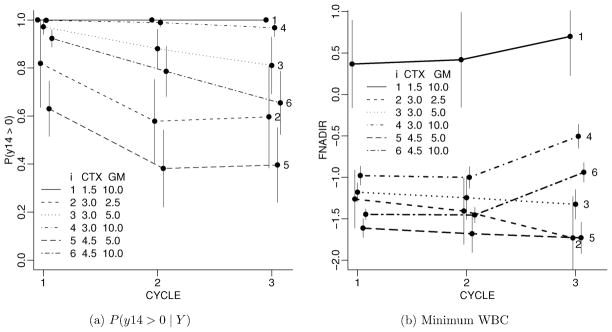
We discuss inference for data with repeated measurements at multiple levels. The motivating example is data with blood counts from cancer patients undergoing multiple cycles of chemotherapy, with days nested within cycles. Some inference questions relate to repeated measurements over days within cycle, while other questions are concerned with the dependence across cycles. When the desired inference relates to both levels of repetition, it becomes important to reflect the data structure in the model. We develop a semiparametric Bayesian modeling approach, restricting attention to two levels of repeated measurements. For the top-level longitudinal sampling model we use random effects to introduce the desired dependence across repeated measurements. We use a nonparametric prior for the random effects distribution. Inference about dependence across second-level repetition is implemented by the clustering implied in the nonparametric random effects model. Practical use of the model requires that the posterior distribution on the latent random effects be reasonably precise.

Figure 1

Model structure. Circles indicate random variables. Arrows indicate conditional dependence. The dashed box and the solid lines (without arrows) show how μ_i is partitioned into subvectors. The sampling model p(y_ijk |θ_ij ), the random effects model p(θ_ij, j = 1, …, n_i | G), and the nonparametric prior p(G |η) are defined in (1), (3), and (5), respectively.

Figure 2

Repeated measurements over time (DAY) and cycles. Each panel shows data for one patient. Within each panel, the curves labeled 1, 2, and 3 show profiles for the first, second, and third cycle of chemotherapy (only two cycles are recorded for patients 15 and 17). The curves show posterior estimated fitted profiles. The observed data are indicated by “1,” “2,” or “3” for cycles 1, 2, and 3, respectively.

Figure 3

Prediction for future patients treated at different levels of CTX and GM-CSF. For each patient we show the predicted response over the first three cycles as solid, dashed, and dotted lines, respectively. CTX levels are 1.5, 3.0, and 4.5 g/m² (labeled as 1, 3, and 4 in the figure). GM-CSF doses are 2.5, 5, and 10 μg/kg (labeled as 3, 5, and 10). Inference is conditional on a baseline of 2.0. Posterior predictive standard deviations are approximately 0.6.

Figure 4

Clinically relevant summaries of the inference across cycles: probability of WBC > 1000 on day 14 (left panel) and estimated nadir WBC count (right panel). The left panel shows the posterior probability of WBC above 1000 on day 14, plotted by treatment and cycle. The right panel shows the minimum WBC (in log 1000) plotted by treatment and cycle. Reported CTX doses are in g/m² and GM-CSF doses are in μg/kg. The vertical error bars show plus/minus 1/2 pointwise posterior predictive standard deviation. We added a small horizontal offset to each line to avoid overlap.

Figure 5

Estimated H(θ). We show the bivariate marginals for cycles 1 and 2 for two relevant summaries of, for doses CTX = 3 g/m² and GM-CSF = 5 μg/kg. (a) shows the estimated distribution of T_lo, the number of days that WBC is below 1000, for the first two cycles. (b) shows the same for the minimum WBC (in log 1000). (c) shows the same inference as (b) for the parametric model. The distributions are represented by scatterplots of 500 simulated draws. For the integer valued variable T_lo we added additional noise to the draws to visualize multiple draws at the same integer pairs. For comparison, the 45 degree line is shown (dashed line).

References

1. Antoniak CE. Mixtures of Dirichlet processes with applications to Bayesian nonparametric problems. Annals of Statistics. 1974;2:1152–1174.
1. Browne WJ, Draper D, Goldstein H, Rasbash J. Bayesian and likelihood methods for fitting multilevel models with complex level-1 variation. Computational Statistics and Data Analysis. 2002;39:203–225.
1. Bush CA, MacEachern SN. A semiparametric Bayesian model for randomised block designs. Biometrika. 1996;83:275–285.
1. Denison D, Holmes C, Mallick B, Smith A. Bayesian Methods for Nonlinear Classification and Regression. New York: Wiley; 2002.
1. Ferguson TS. A Bayesian analysis of some nonparametric problems. Annals of Statistics. 1973;1:209–230.
Publication types