. 2007 May 1;104(18):7332-6.
doi: 10.1073/pnas.0610245104. Epub 2007 Apr 24.

Structure and tie strengths in mobile communication networks

Affiliations

Structure and tie strengths in mobile communication networks

J-P Onnela et al. Proc Natl Acad Sci U S A. .

Abstract

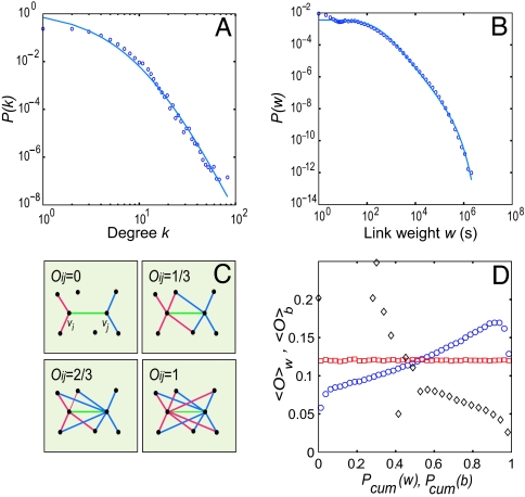
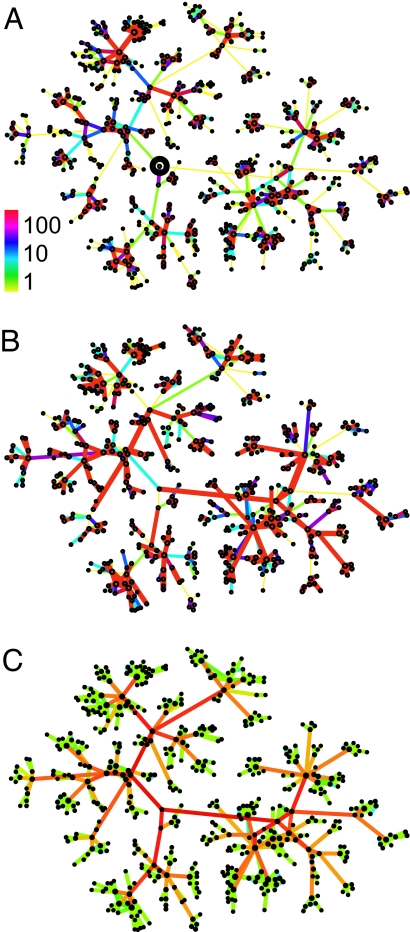
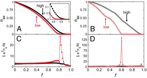
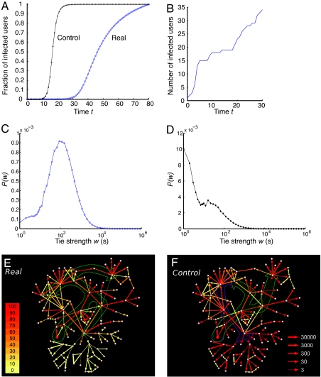
Electronic databases, from phone to e-mails logs, currently provide detailed records of human communication patterns, offering novel avenues to map and explore the structure of social and communication networks. Here we examine the communication patterns of millions of mobile phone users, allowing us to simultaneously study the local and the global structure of a society-wide communication network. We observe a coupling between interaction strengths and the network's local structure, with the counterintuitive consequence that social networks are robust to the removal of the strong ties but fall apart after a phase transition if the weak ties are removed. We show that this coupling significantly slows the diffusion process, resulting in dynamic trapping of information in communities and find that, when it comes to information diffusion, weak and strong ties are both simultaneously ineffective.


Conflict of interest statement

Conflict of interest statement: A.L.B. served as a paid consultant for the phone company that provided the phone data.

Figures

Fig. 1.
Fig. 1.
Characterizing the large-scale structure and the tie strengths of the mobile call graph. (A and B) Vertex degree (A) and tie strength distribution (B). Each distribution was fitted with P(x) = a(x + x0)x exp(−x/xc), shown as a blue curve, where x corresponds to either k or w. The parameter values for the fits are k0 = 10.9, γk = 8.4, kc = ∞ (A, degree), and w0 = 280, γw = 1.9, wc = 3.45 × 10⁵ (B, weight). (C) Illustration of the overlap between two nodes, vi and vj, its value being shown for four local network configurations. (D) In the real network, the overlap 〈Ow (blue circles) increases as a function of cumulative tie strength Pcum(w), representing the fraction of links with tie strength smaller than w. The dyadic hypothesis is tested by randomly permuting the weights, which removes the coupling between 〈O〉w and w (red squares). The overlap 〈Ob decreases as a function of cumulative link betweenness centrality b (black diamonds).
Fig. 2.
Fig. 2.
The structure of the MCG around a randomly chosen individual. Each link represents mutual calls between the two users, and all nodes are shown that are at distance less than six from the selected user, marked by a circle in the center. (A) The real tie strengths, observed in the call logs, defined as the aggregate call duration in minutes (see color bar). (B) The dyadic hypothesis suggests that the tie strength depends only on the relationship between the two individuals. To illustrate the tie strength distribution in this case, we randomly permuted tie strengths for the sample in A. (C) The weight of the links assigned on the basis of their betweenness centrality bij values for the sample in A as suggested by the global efficiency principle. In this case, the links connecting communities have high bij values (red), whereas the links within the communities have low bij values (green)..
Fig. 3.
Fig. 3.
The stability of the mobile communication network to link removal. The control parameter f denotes the fraction of removed links. (A and C) These graphs correspond to the case in which the links are removed on the basis of their strengths (wij removal). (B and D) These graphs correspond to the case in which the links were removed on the basis of their overlap (Oij removal). The black curves correspond to removing first the high-strength (or high Oij) links, moving toward the weaker ones, whereas the red curves represent the opposite, starting with the low-strength (or low Oij) ties and moving toward the stronger ones. (A and B) The relative size of the largest component RGC(f) = NGC(f)/NGC(f = 0) indicates that the removal of the low wij or Oij links leads to a breakdown of the network, whereas the removal of the high wij or Oij links leads only to the network's gradual shrinkage. (A Inset) Shown is the blowup of the high wij region, indicating that when the low wij ties are removed first, the red curve goes to zero at a finite f value. (C and D) According to percolation theory, = Σ s<smaxnss2/N diverges for N → ∞ as we approach the critical threshold fc, where the network falls apart. If we start link removal from links with low wij (C) or Oij (D) values, we observe a clear signature of divergence. In contrast, if we start with high wij (C) or Oij (D) links, there the divergence is absent. Finite size scaling shows that the small local maximum seen in D at f ≈ 0.95 does not correspond to a real phase transition (see SI Appendix).
Fig. 4.
Fig. 4.
The dynamics of spreading on the weighted mobile call graph, assuming that the probability for a node vi to pass on the information to its neighbor vj in one time step is given by Pij = xwij, with x = 2.59 × 10⁻⁴. (A) The fraction of infected nodes as a function of time t. The blue curve (circles) corresponds to spreading on the network with the real tie strengths, whereas the black curve (asterisks) represents the control simulation, in which all tie strengths are considered equal. (B) Number of infected nodes as a function of time for a single realization of the spreading process. Each steep part of the curve corresponds to invading a small community. The flatter part indicates that the spreading becomes trapped within the community. (C and D) Distribution of strengths of the links responsible for the first infection for a node in the real network (C) and control simulation (D). (E and F) Spreading in a small neighborhood in the simulation using the real weights (E) or the control case, in which all weights are taken to be equal (F). The infection in all cases was released from the node marked in red, and the empirically observed tie strength is shown as the thickness of the arrows (right-hand scale). The simulation was repeated 1,000 times; the size of the arrowheads is proportional to the number of times that information was passed in the given direction, and the color indicates the total number of transmissions on that link (the numbers in the color scale refer to percentages of 1,000). The contours are guides to the eye, illustrating the difference in the information direction flow in the two simulations.

References

    1. Ebel H, Mielsch L-I, Bornholdt S. Phys Rev E Stat Phys Plasmas Fluids Relat Interdiscip Top. 2002;66:35103. - PubMed
    1. Eckmann J-P, Moses E, Sergi D. Proc Natl Acad Sci USA. 2004;101:14333–14337. - PMC - PubMed
    1. Dodds PS, Muhamad R, Watts DJ. Science. 2003;301:827–829. - PubMed
    1. Aiello W, Chung F, Lu L. Proceedings of the 32nd ACM Symposium on the Theory of Computing; New York: Assoc Comput Machinery; 2000. pp. 171–180.
    1. Wasserman S, Faust K. Social Network Analysis: Methods and Applications. Cambridge: Cambridge Univ Press; 1994.

Publication types

LinkOut - more resources