Is matching innate?

Abstract

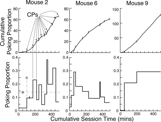
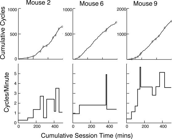
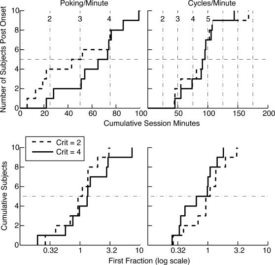
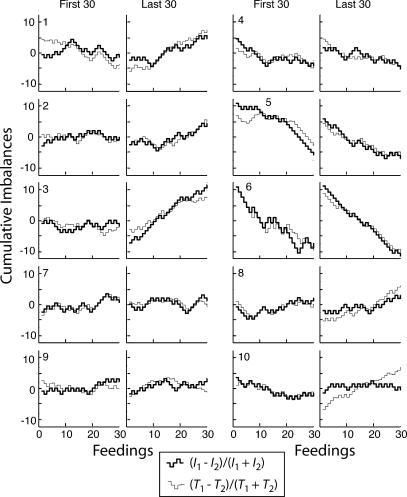
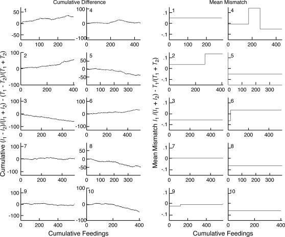
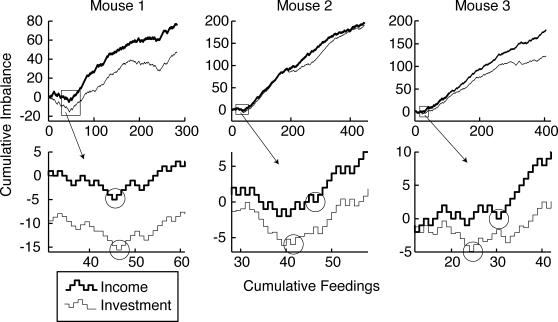
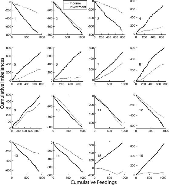
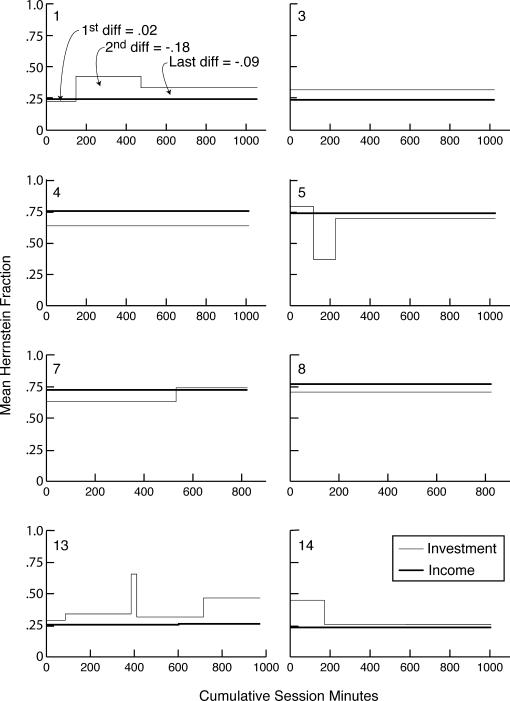
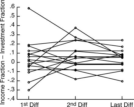
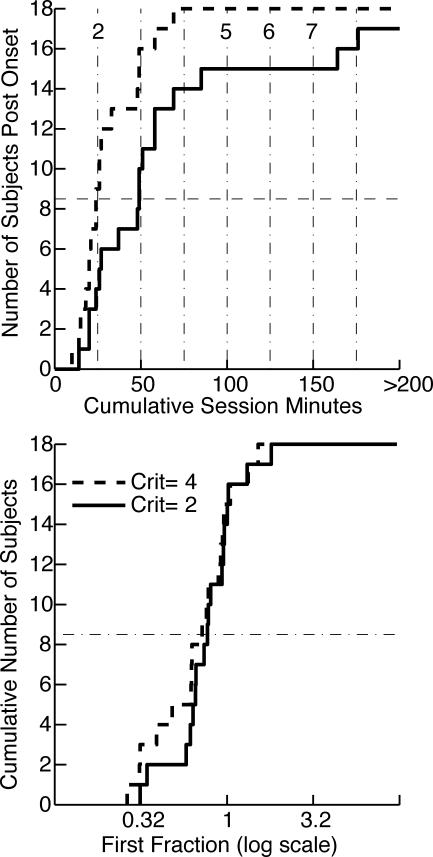
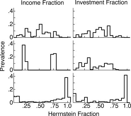
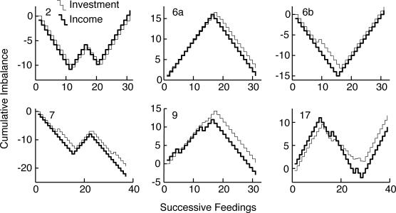
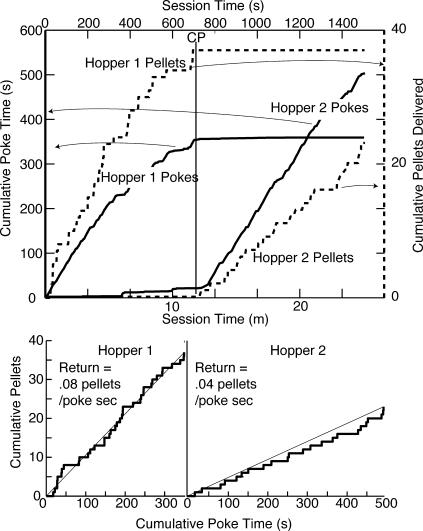
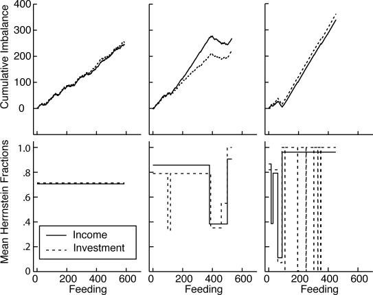
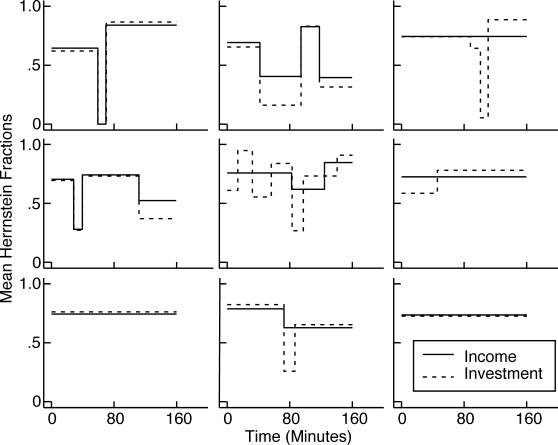
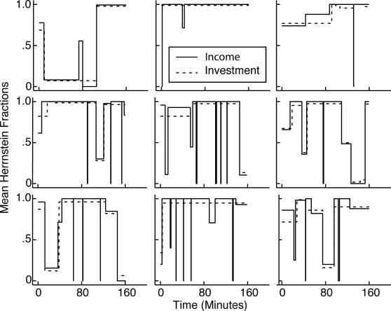
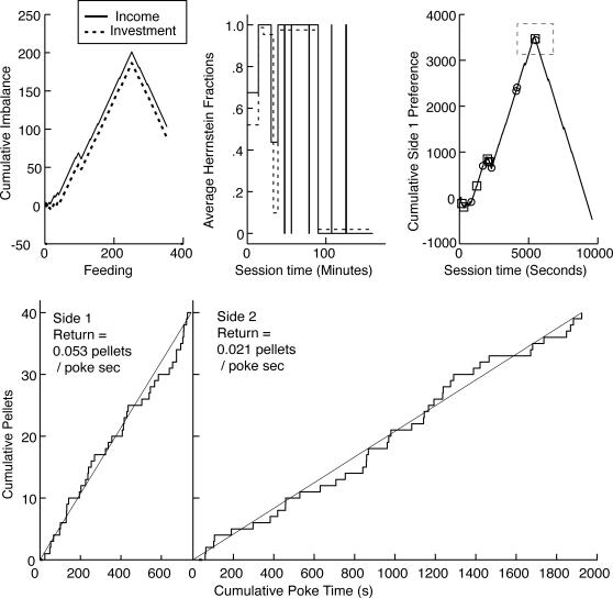
Experimentally naive mice matched the proportions of their temporal investments (visit durations) in two feeding hoppers to the proportions of the food income (pellets per unit session time) derived from them in three experiments that varied the coupling between the behavioral investment and food income, from no coupling to strict coupling. Matching was observed from the outset; it did not improve with training. When the numbers of pellets received were proportional to time invested, investment was unstable, swinging abruptly from sustained, almost complete investment in one hopper, to sustained, almost complete investment in the other-in the absence of appropriate local fluctuations in returns (pellets obtained per time invested). The abruptness of the swings strongly constrains possible models. We suggest that matching reflects an innate (unconditioned) program that matches the ratio of expected visit durations to the ratio between the current estimates of expected incomes. A model that processes the income stream looking for changes in the income and generates discontinuous income estimates when a change is detected is shown to account for salient features of the data.

Fig 1. Cumulative number of pellets obtained as a function of time.

The change-detecting algorithm operates on this function, as it evolves. In this instance, with simulated data, its evolution spans a step change in the underlying random rate. The current moment is t; the no-change (constant rate) hypothesis is represented by the thin straight line from the origin to the current value of n(t); τ_m is the past moment at which n(t) deviates maximally from the value expected on the constant-rate hypothesis.

Fig 2. Top row: Representative minute-by-minute cumulative records of poking proportion (proportion of each minute during which an infrared beam was interrupted) for 3 representative mice.

The small ovals (CPs) mark the change points found by the change-point algorithm with a logit decision criterion of 4. Bottom row: The slopes of the straight-line segments connecting the change points. These slopes are the mean poking proportion during the successive segments of the parsed cumulative record. Bottom left panel: a  =  average poking proportion during the last 10 sessions; o = onset of conditioned poking; f  =  mean poking proportion for the first segment after the onset. The f/a ratio is the first fraction, a measure of the abruptness of a change.

Fig 3. Upper row: Representative cumulative records of the number of visit cycles as a function of session time, parsed by the change-point algorithm with a logit decision criterion of 4 (small ovals).

Lower row: Slopes of successive segments of the cumulative record. These slopes are the average cycles per min.

Fig 4. Cumulative distributions of onset latencies and first fractions (the poking proportion immediately after the first increase divided by the asymptotic poking proportion) for poking proportions (poking per min) and cycling rates (cycles per min).

A cumulative distribution shows the number of subjects giving the value on the x axis or less. The x axis value at each upward step gives the datum for one subject. The solid lines are the distributions when a conservative decision criterion is used to parse the cumulative records; the dashed lines are the distributions when a hundredfold-more-sensitive criterion is used. A dashed horizontal line is drawn at 5 to aid in extracting the medians, which are the values on the abscissa at which the cumulative distributions cross this line. In the upper panels, the numbered vertical dashed lines indicate session boundaries. Crit  =  logit decision criterion used in parsing the cumulative records.

Fig 5. Cumulative records of the feeding-by-feeding income imbalance (heavy lines) and the investment imbalance (light lines) for the first 30 and last 30 feedings.

The imbalance is the difference between two complementary Herrnstein fractions. The number in the upper or lower left corner of the “First 30” panels identifies the subject. For Subjects 1–3, the concurrent random-interval schedules favored Hopper 1 by 3∶1; for Subjects 4–6, they favored Hopper 2, by 3∶1; for Subjects 7–10, the schedule ratio was 1∶1. These records are a sequence of steps because at this resolution one sees every feeding. The imbalances are only recomputed at each feeding, so their cumulative record is flat between feedings and steps up or down at each feeding.

Fig 6. Left: Cumulative feeding-by-feeding difference between the income imbalance and the investment imbalance.

The number in the upper left corner of each panel identifies the subject. The y axis has been scaled so that a difference equivalent to an average difference in the Herrnstein fractions (average mismatch) of .125 would produce a full-scale deflection by the end of the record. Right: Plots of the slopes of the cumulative difference records when parsed with a logit decision criterion of 2. The y axis has been scaled in terms of the difference in the Herrnstein fractions (average mismatch). Positive mismatches constitute overmatching for the subjects whose schedules favored Hopper 1 (Subjects 1–3) and undermatching for those whose schedules favored Hopper 2 (Subjects 4–6).

Fig 7. Cumulative records of the feeding-by-feeding income and investment imbalances for Subjects 1–3.

Upper row: Complete records. Lower row: Thirty feedings surrounding the initial change in slope. Circles indicate the loci of the change points found by the parsing algorithm. For the binary-valued data in the records of income imbalance, the parsing algorithm used the chi square test to compare the proportion of +1 imbalances (feedings at Hopper 1) to the proportion of −1 imbalances (feedings at Hopper 2) before and after a putative change point. For the real-valued and not normally distributed data in the records of investment imbalance, it used the two-sample Kolmogorov-Smirnov test.

Fig 8. Cumulative distribution of onset latencies (top panels) and first fractions (bottom panels).

(The first fraction is the poking proportion immediately after the first increase divided by the asymptotic poking proportion.) Crit  =  logit decision criterion used in parsing the cumulative records. Dashed vertical lines in top panels are session boundaries. Dashed horizontal lines at the bisection point on the y axis are aids to the extraction of the medians.

Fig 9. Cumulative feeding-by-feeding imbalance records from Experiment 2.

Heavy lines  =  income imbalance; light lines  =  investment imbalance. Numbers at middle-left identify the subjects.

Fig 10. Successive mean Herrnstein income and investment fractions for the 8 mice that matched only approximately, as determined by the parsing algorithm with a decision criterion of 4.

(Four other mice matched almost exactly throughout; and 3 did not match during all or most of training—see Figure 9.) The upper left panel gives the first, second, and last mismatch (income fraction minus investment fraction). The numbers in the upper left corners identify the subjects.

Fig 11. First, second, and last mismatches (income fraction minus investment fraction).

Fig 12. Top panel: Cumulative distribution of the time at which the first increase in poking proportion occurred, for two different parsing criteria.

The dashed vertical lines indicate session boundaries. Bottom panel: Cumulative distribution of first fractions. (The first fraction is the poking proportion immediately after the first increase divided by the asymptotic poking proportion.)

Fig 13. The prevalence of the income and investment fractions in the three experiments.

Prevalence is the fraction of the total time that a given range of fractions prevailed. Ranges are in bins of .05.

Fig 14. Cumulative income and investment imbalance records.

Where only the income record is apparent, it is obscuring the investment record. The number at upper or lower left of a panel identifies the subject. For Subjects 2, 6, 7, 9, and 17, thin rectangles superposed on abrupt slope reversals indicate the portions of the records shown at high resolution in Figure 15.

Fig 15. High-resolution cumulative imbalance records covering abrupt reversals.

The numbers inside the panels identify the subject. The portions of the complete records from which these come are indicated by small superposed rectangles in Figure 14. Each step in one of these records corresponds to a single feeding. Where necessary, the records have been vertically displaced to superpose them, facilitating comparison of their slopes.

Fig 16. Analysis of an abrupt reversal in Subject 6.

Upper panel plots the cumulative record of poke durations in the two hoppers (solid lines, left ordinate) and the cumulative record of pellet deliveries (dashed lines, right ordinate), as functions of session time. The vertical line in the middle of the plot indicates the point at which the investments in, and incomes from the two hoppers abruptly reversed. This point of reversal is the vertical line more or less in the middle of the lower panel. To the left of this reversal point, the lower panel plots the cumulative record of pellet deliveries against cumulative poke time in Hopper 1 up to the point of reversal; to the right, the lower panel plots the cumulative record of pellet deliveries in Hopper 2 against poke time in Hopper 2 after the point of reversal. Thin straight lines connect the origins of these records to their end points. The slopes of these lines are the average returns (pellets per s invested in a hopper). Note that the slope of the record on the right (the return from Hopper 2) is everywhere less than the slope of the record on the left (the return from Hopper 1).

Fig 17. Examples of maximally abrupt reversals.

The investment imbalance (heavy solid line, right ordinate) is plotted against the cumulative investment (cumulative duration of the stays on both sides). Each plot shows a fragment that includes one or more shifts from one extreme to the other in the span of one or two visit cycles. Each step in these stair plots represents the investment imbalance during one visit cycle (consisting of a stay at each hopper). If the step's elevation is close to +1, the investment was almost entirely in Hopper 1; if it is close to −1, the investment was almost entirely in Hopper 2. The width of a step is the total investment on that cycle, that is, the combined duration of the two stays, one at each hopper. The two light lines plot the cumulative excess of the investment in one side over the investment in the other, again as a function of the total investment. The cumulative excess is positive if more time has been spent at Hopper 1 and negative if more time has been spent at Hopper 2. The cumulative excess is plotted either as a continuous function of the cumulative investment (dashed light line) or a step function of the cumulative investment (solid light line). In the latter case, the plot steps at the end of each visit cycle, which is the point at which the excess for that cycle is computed. (The aforementioned heavy line is the discrete derivative of this step plot—the ratio of the signed excess on that visit to the total investment on that visit.) The number at the top of each plot identifies the subject.

Fig 18. Representative simulations under three conditions.

Top panels: Cumulative records of feeding-by-feeding income and preference differences. Bottom panels: Mean Herrnstein fraction between change points, after parsing cumulative records with a logit decision criterion equal to 2. Left: Income independent of behavioral investment, no change-detection mechanism. Middle: Income independent of investment, change-detecting mechanism added. Right: Income proportional to behavioral investment, with change detection.

Fig 19. Between-change-point Herrnstein fractions at the richer location in nine random simulations, with income independent of behavioral investment.

Change-point logit criterion  =  2. Hoppers 1 and 2 delivered rewards on RI 20-s and RI 40-s schedules, respectively.

Fig 20. Between-change-point Herrnstein fractions at the richer location in nine random simulations, with income proportional to behavioral investment.

Change-point logit criterion  =  2. Hoppers 1 and 2 delivered rewards on RI 20-s and RI 40-s schedules, respectively, where I is the time on the clock that ran only when the head was in that hopper.

Fig 21. A simulation under the conditions of Experiment 3.

Top Left Panel: Cumulative record of feeding-by-feeding income and preference differences. Top Middle Panel: Between-change-point Herrnstein fractions for income and preference. Top Right Panel: Second-by-second cumulative record of investment imbalance (preference) for the rich hopper (Hopper 1). Preference is 1 if the second was spent at the richer location and −1 if it was spent at the leaner location. Open circles mark changes in income estimates for the richer location. Open squares mark changes in income estimates for the poorer location. The dashed rectangle indicates the period covered by the plots of returns in the lower panels. Bottom Left Panel: Cumulative feeding-by-feeding return for the 40 richer location feedings that preceded the switch to the poorer location. Bottom Right Panel: Cumulative return for the 40 poorer location feedings that followed the switch. The schedules for Hoppers 1 and 2 delivered rewards on RI 20-s and RI 40-s schedules, respectively, where I is the time on the clock that ran only when the head was in that hopper.

References

1. Balsam P.D, Fairhurst S, Gallistel C.R. Unsignaled unconditioned stimuli degrade contingencies by changing cycle time and temporal uncertainty. Journal of Experimental Psychology: Animal Behavior Processes in press. - PubMed
1. Belke T.W. Stimulus preference and the transitivity of preference. Animal Learning & Behavior. 1992;20:401–406.
1. Bush R.R, Mosteller F. A mathematical model for simple learning. Psychological Review. 1951;58:313–323. - PubMed
1. Catania A.C. Concurrent performances: A baseline for the study of reinforcement magnitude. Journal of the Experimental Analysis of Behavior. 1963;6:299–300. - PMC - PubMed
1. Church R.M, Guilhardi P. A Turing test of a timing theory. Behavioural Processes. 2005;69:45–58. - PubMed
Publication types
LinkOut - more resources