. 2007 Jul;176(3):1635-51.
doi: 10.1534/genetics.107.072371. Epub 2007 May 4.

A Markov chain Monte Carlo approach for joint inference of population structure and inbreeding rates from multilocus genotype data

Affiliations

A Markov chain Monte Carlo approach for joint inference of population structure and inbreeding rates from multilocus genotype data

Hong Gao et al. Genetics. 2007 Jul.

Abstract

Nonrandom mating induces correlations in allelic states within and among loci that can be exploited to understand the genetic structure of natural populations (Wright 1965). For many species, it is of considerable interest to quantify the contribution of two forms of nonrandom mating to patterns of standing genetic variation: inbreeding (mating among relatives) and population substructure (limited dispersal of gametes). Here, we extend the popular Bayesian clustering approach STRUCTURE (Pritchard et al. 2000) for simultaneous inference of inbreeding or selfing rates and population-of-origin classification using multilocus genetic markers. This is accomplished by eliminating the assumption of Hardy-Weinberg equilibrium within clusters and, instead, calculating expected genotype frequencies on the basis of inbreeding or selfing rates. We demonstrate the need for such an extension by showing that selfing leads to spurious signals of population substructure using the standard STRUCTURE algorithm with a bias toward spurious signals of admixture. We gauge the performance of our method using extensive coalescent simulations and demonstrate that our approach can correct for this bias. We also apply our approach to understanding the population structure of the wild relative of domesticated rice, Oryza rufipogon, an important partially selfing grass species. Using a sample of n = 16 individuals sequenced at 111 random loci, we find strong evidence for existence of two subpopulations, which correlates well with geographic location of sampling, and estimate selfing rates for both groups that are consistent with estimates from experimental data (s approximately 0.48-0.70).


Figures

F<sc>igure</sc> 1.—
Figure 1.—
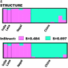
Population assignments for a single data set of 100 individuals simulated under partial selfing (s = 50%) and no population substructure and analyzed assuming K = 2. (a and b) The Distruct graph from STRUCTURE using (a) the correlated alleles model and (b) the uncorrelated alleles model. (c) The Distruct graph from InStruct of the same data set. (d) Distribution of log-likelihood difference between the K = 2 and the K = 1 model under six levels of population selfing rates as estimated by STRUCTURE using the F model (A)/InStruct (B). Each colored line represents the density of average log-likelihood difference with 100 replicate data sets simulated without population structure and under a specific selfing rate, indicated in the inset.
F<sc>igure</sc> 2.—
Figure 2.—
The posterior distribution of selfing rates estimated from simulations without population structure under six levels of population selfing rates. Each colored line represents the density of the posterior mean of selfing rates of 100 simulation runs under a specific selfing rate in the key.
F<sc>igure</sc> 3.—
Figure 3.—
The posterior distribution of selfing rates estimated from simulations under model 2 with six combinations of selfing rates: (A) s = {0.0, 0.3}, (B) s = {0.0, 0.9}, (C) s = {0.3, 0.3}, (D) s = {0.3, 0.6}, (E) s = {0.3, 0.9}, and (F) s = {0.9, 0.9}. Each colored line represents the density of the posterior mean of a subpopulation selfing rate from 100 simulation runs under a specific combination of selfing rates in the key.
F<sc>igure</sc> 4.—
Figure 4.—
The posterior distribution of selfing rates estimated from simulations under model 3 with six combinations of selfing rates: (A) S = {0.4, 0.5, 0.6}, (B) S = {0.1, 0.5, 0.9}, (C) S = {0.1, 0.1, 0.1}, (D) S = {0.25, 0.6, 0.85}, (E) S = {0.05, 0.45, 0.75}, and (F) S = {0.9, 0.9, 0.9}. Each colored line represents the density of the posterior mean of a subpopulation selfing rate from 100 data sets simulated under a specific selfing rate combination in the key.
F<sc>igure</sc> 5.—
Figure 5.—
The posterior distribution of selfing rates estimated from simulations with six subpopulations of unequal selfing rates. Each colored line represents the density of the posterior mean of a subpopulation selfing rate from 50 simulation runs under a specific selfing rate in the key.
F<sc>igure</sc> 6.—
Figure 6.—
The distributions of posterior medians of selfing rates of 100 individuals drawn from the Dirichlet process mixture model. The magenta dashed lines represent the true distribution of selfing rates in the simulation. The red, green, blue, and yellow solid lines are the estimated densities from the Dirichlet process mixture model with scaling parameters α = 1, α = 5, α = 10, and α = 20, respectively. The individual selfing rates were simulated under three different scenarios in three columns: (1) model ident (A) S = 0.3 and (D) S = 0.7, (2) model norm (B) formula image and (E) formula image, and (3) model beta (C) S ∼ beta(9, 3) and (F) S ∼ beta(10, 25).
F<sc>igure</sc> 7.—
Figure 7.—
(a) The Distruct plot of population assignment for n = 16 rice accessions assuming K = 2 from STRUCTURE and InStruct. The two clusters are represented by pink and light blue. For InStruct, the corresponding selfing rates of subpopulations are indicated at the top. (b) Estimated selfing rates under the individual model using the Dirichlet process prior model. The points represent the posterior mean of individual selfing rates and their different shapes indicate the countries where that individual was collected: squares with x's inside represent China, diamonds represent Nepal, circles represent India, and triangles indicate Laos. The x-axis represents the index of 16 individuals collected from the wild. The red lines across the points represent the 90% posterior confidence intervals of individual selfing rates.

Similar articles

Cited by

References

    1. Ayres, K. L., and D. J. Balding, 1998. Measuring departures from Hardy-Weinberg: a Markov chain Monte Carlo method for estimating the inbreeding coefficient. Heredity 80(6): 769–777. - PubMed
    1. Corander, J., P. Waldmann and M. Sillanpaa, 2003. Bayesian analysis of genetic differentiation between populations. Genetics 163: 367–374. - PMC - PubMed
    1. Dawson, K. J., and K. Belkhir, 2001. A Bayesian approach to the identification of panmictic populations and the assignment of individuals. Genet. Res. 78: 59–77. - PubMed
    1. Enjalbert, J., and J. L. David, 2000. Inferring recent outcrossing rates using multilocus individual heterozygosity: application to evolving wheat populations. Genetics 156: 1973–1982. - PMC - PubMed
    1. Falush, D., M. Stephens and J. K. Pritchard, 2003. Inference of population structure using multilocus genotype data: linked loci and correlated allele frequencies. Genetics 164: 1567–1587. - PMC - PubMed

Publication types