Bayesian multiple quantitative trait loci mapping for complex traits using markers of the entire genome

Abstract

A Bayesian methodology has been developed for multiple quantitative trait loci (QTL) mapping of complex binary traits that follow liability threshold models. Unlike most QTL mapping methods where only one or a few markers are used at a time, the proposed method utilizes all markers across the genome simultaneously. The outperformance of our Bayesian method over the traditional single-marker analysis and interval mapping has been illustrated via simulations and real data analysis to identify candidate loci associated with colorectal cancer.

Figure 1.—

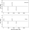
Bayesian estimates of QTL effects in the simulated backcross family under setup one. (a) Results from (underlying) normal liability data and (b) results from binary data. “x” refers to the simulated QTL position (x-axis) and effect (y-axis). The 95% confidence interval is bracketed by two horizontal lines. The heights of the solid lines correspond to the posterior means.

Figure 2.—

Histograms for the posterior QTL effects at the four simulated markers for binary data (left) and normal data (right).

Figure 3.—

Estimates of QTL effects in the simulated backcross family (n = 300) with 11 QTL of different genetic effects. (a) Single-marker analysis based on a chi-square test; (b) Bayesian analysis. “x” refers the simulated QTL position (x-axis) and effect (y-axis). The 95% confidence interval is bracketed by two horizontal lines. The heights of the solid lines in b correspond to the posterior means.

Figure 4.—

Estimates of QTL effects in the simulated backcross family (n = 500) with 11 QTL of different genetic effects. (a) Single-marker analysis based on chi-square test; (b) Bayesian analysis. “x” refers the simulated QTL position (x-axis) and effect (y-axis). The 95% confidence interval is bracketed by two horizontal lines. The heights of the solid lines in b correspond to the posterior means.

Figure 5.—

Number of tumors in two parental strains A/J and SPRET/EiJ, plus ASP F₁ and backcross strains.

Figure 6.—

(a) Bayesian analysis; (b) single-marker analysis based on a chi-square test. Vertical dotted lines are used to separate the chromosomes. The 95% confidence intervals are bracketed by x's and shown at the two positions with the highest posterior means. The heights of the solid lines in a correspond to the posterior means.

Figure 7.—

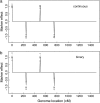
Bayesian estimates of QTL effects in the simulated backcross family with four QTL for continuous and binary data. “x” refers the simulated QTL position (x-axis) and effect (y-axis). The 95% confidence interval is bracketed by two horizontal lines. The heights of the solid lines correspond to the posterior means.

Figure 8.—

Bayesian estimates of QTL effects in the simulated backcross family x with 20 QTL for continuous and binary data. The heights of the solid lines correspond to the posterior means. “x” refers to the simulated QTL position (x-axis) and effect (y-axis).

Figure 9.—

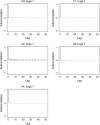
Autocorrelation function for the study of setup one. Here b0 represents μ and b1–b4 represent the effects of four markers at which the true QTL are located.

Figure 10.—

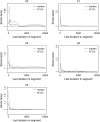
Plot of Gelman and Rubin's shrink factor for the study of setup one. Here b0 represents μ and b1–b4 represent the effects of four markers at which the true QTL are located.

References

1. Best, N. C., M. K. Cowles and S. K. Vines, 1995. CODA Manual Version 0.30. MRC Biostatistics Unit, Cambridge, UK.
1. Carlborg, O., and L. Andersson, 2002. Use of randomization testing to detect multiple epistatic QTL. Genet. Res. 79: 175–184. - PubMed
1. Coffman, C. J., R. W. Doerge, K. L. Simonsen, K. M. Nichols, C. K. Duarte et al., 2005. Model selection in binary trait locus mapping. Genetics 170: 1281–1297. - PMC - PubMed
1. Falconer, D. S., 1965. The inheritance of liability to certain diseases, estimated from the incidence among relatives. Ann. Hum. Genet. 29: 51–71.
1. Falconer, D. S., and T. F. C. Mackay, 1996. Introduction to Quantitative Genetics, Ed. 4. Addison-Wesley, Boston.
Publication types