AIDA: an adaptive image deconvolution algorithm with application to multi-frame and three-dimensional data

Abstract

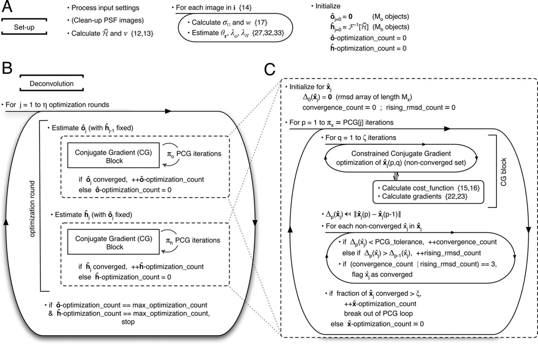
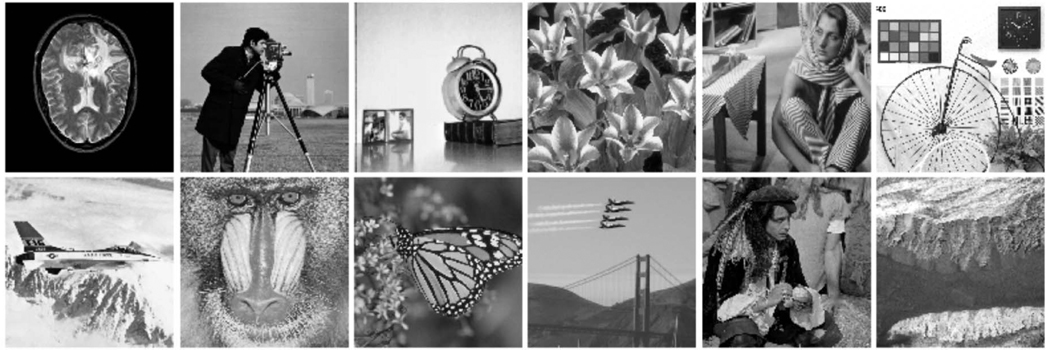
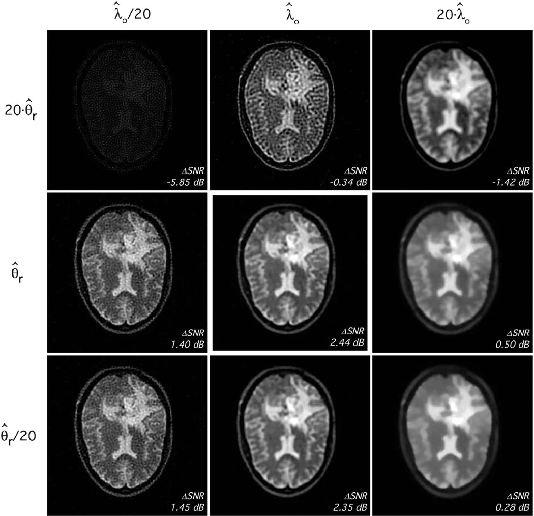
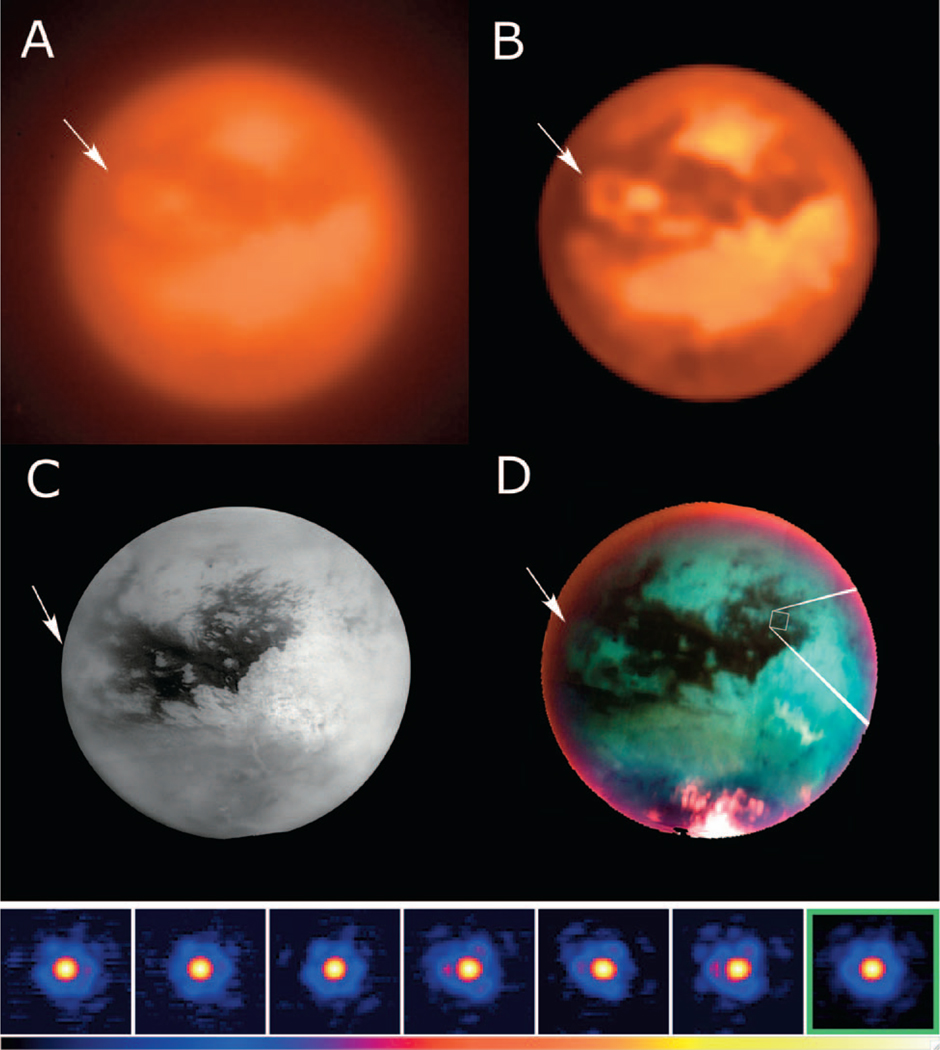
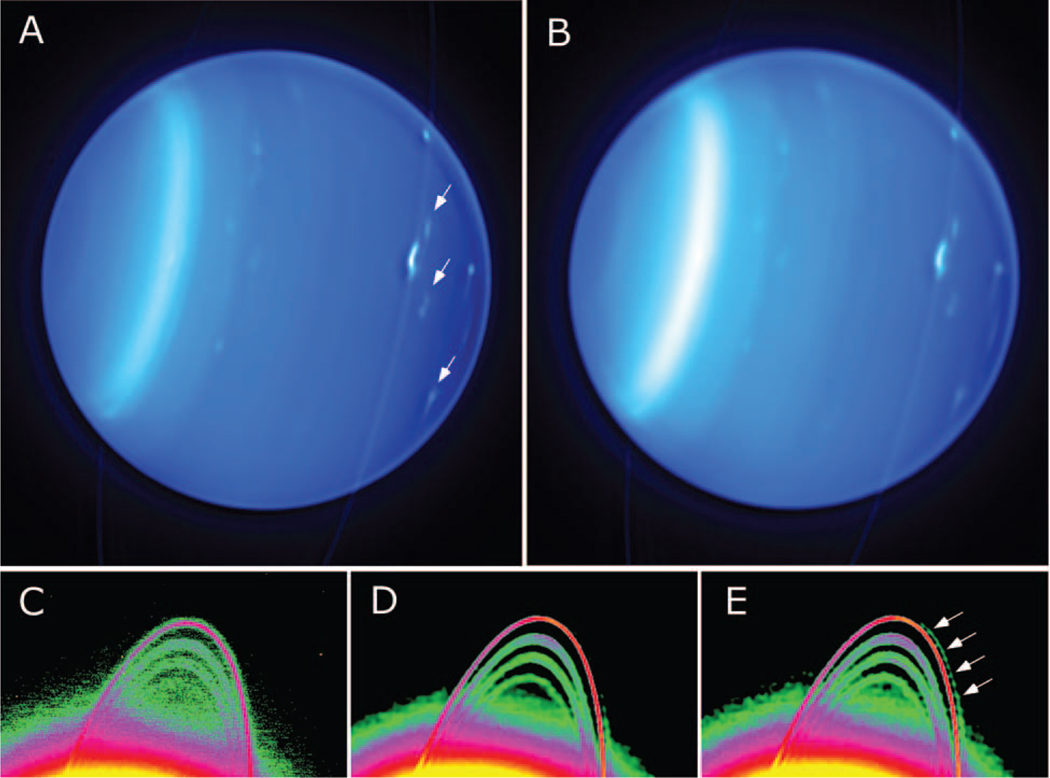
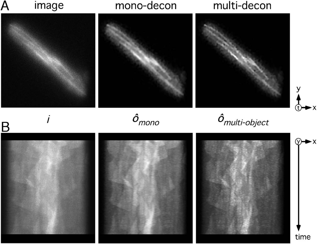
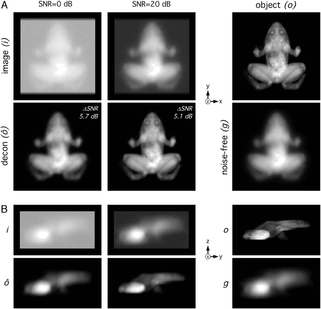
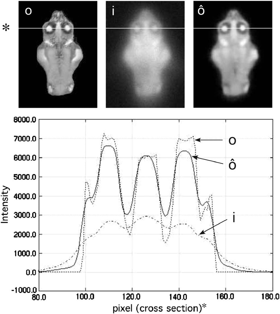
We describe an adaptive image deconvolution algorithm (AIDA) for myopic deconvolution of multi-frame and three-dimensional data acquired through astronomical and microscopic imaging. AIDA is a reimplementation and extension of the MISTRAL method developed by Mugnier and co-workers and shown to yield object reconstructions with excellent edge preservation and photometric precision [J. Opt. Soc. Am. A21, 1841 (2004)]. Written in Numerical Python with calls to a robust constrained conjugate gradient method, AIDA has significantly improved run times over the original MISTRAL implementation. Included in AIDA is a scheme to automatically balance maximum-likelihood estimation and object regularization, which significantly decreases the amount of time and effort needed to generate satisfactory reconstructions. We validated AIDA using synthetic data spanning a broad range of signal-to-noise ratios and image types and demonstrated the algorithm to be effective for experimental data from adaptive optics-equipped telescope systems and wide-field microscopy.

Fig. 1

AIDA optimization protocol. A: Setup and variable initialization stage. Equation numbers for variables are shown in curly brackets. M_o and M_h are the number of objects and PSFs to be estimated, respectively. B: Deconvolution scheme. The subscript j indexes the optimization round, which consists of two partial conjugate gradient (PCG) estimation loops (each indicated by a dashed box): one for the object(s), ô, followed by one for the PSF(s), ĥ. The deconvolution is stopped after a max_optimization_count number of sequential PCG estimation loops have converged (see below). C: Schematic of the PCG estimation loop used to estimate the object(s) or PSF(s) [indicated generically by the variable (x̂_j)] for the jth optimization round. Δ_p is an M_o- or M_h-length array of root-mean-square deviations between sequential PCG iterations used to monitor convergence progress. Minimization of each x̂_j in x̂_j is continued until Δ_p falls below some PCG_tolerance for a total of convergence_count times or until a rising_rmsd_count number of uphill moves is registered (default = 3 for both). Each PCG iteration entails a steepest-descent minimization step followed by up to ζ − 1 conjugate gradient (CG) steps for the set of unconverged object or PSF estimates. When the fraction of object(s) or PSF(s) that have converged is >ξ, the PCG estimation is stopped, and convergence for that PCG estimation loop is noted.

Fig. 2

Subset of reference objects used to test AIDA and establish its automatic hyperparameter estimation scheme. Each object (with maximum intensity set to 100, 1000, or 10,000) was blurred with a Gaussian PSF (FWHM = 4 pixels), had intensity-based Poisson noise and Gaussian detector noise added according to Eq. (34) to yield a series of images with SNR = −10, −3, 0, 7, 10, 17, 20, or 27 dB.

Fig. 3

Classical deconvolution test results using automatic hyperparameter estimation. A: Deconvolution series for image SNR of 0, 10, and 20 dB; top, convolved image with Poisson and Gaussian noise (i); bottom, corresponding deconvolution result (ô) and signal-to-noise improvement, ΔSNR [Eq. (36)]. B: Top, original 256 × 256 pixel brain object with intensities from 0–1000 (o); bottom, convolved noise-free image (g) with Gaussian PSF (h) inset (FWHM = 4 pixels).

Fig. 4

Automatic hyperparameter estimates are close to the optimum. Classical deconvolution results for the SNRI = 20 dB brain image from Fig. 3, over a grid of λ_o and θ_r values that are 20× larger or smaller than those estimated automatically. Center: Deconvolution result using the automatically estimated hyperparameters. Signal-to-noise improvements are shown in the lower right of each panel.

Fig. 5

Myopic deconvolution results for a test phantom. A: The original phantom object, o. B: The convolved and noisy phantom image, i (SNR = 17 dB). C: Reconstructed object after classical deconvolution using the average of synthetically generated PSFs (see Fig. 6) (ΔSNR = 1.7 dB). D: Reconstructed object after myopic deconvolution with automatic hyperparameter estimates and the average PSF, h̄, as an initial PSF guess (ΔSNR = 2.9 dB). E: Same as D, except the hyperparameter, λ_o, is scaled to 1/2 of the value of the automatic estimate (ΔSNR = 4.2 dB). F: Reconstructed object after classical deconvolution using the true PSF [see Fig. 6(B)] with the same hyperparameter settings as in (E) (ΔSNR = 3.8 dB).

Fig. 6

PSFs associated with the myopic deconvolution of the test phantom. A: Sample PSFs used to myopically deconvolve the test phantom data of Fig. 5. PSFs were generated as the modulus of the Fourier transfer of pupil functions with random Zernike polynomial phase components of up to order 15 (OSA convention; Gaussian-distributed amplitudes with mean = 0 and standard deviation = 0.1). Resulting PSFs have an average FWHM between 3 and 4 pixels. To simulate typical PSF measurements, Poisson and Gaussian noise was added for a PSF image SNR of 17 dB. B (from left to right): The true PSF, h_true, used to generate Fig. 5(B); the average PSF, h̄, used as the initial guess in myopic deconvolution; the myopically recovered PSF, ĥ, using a harmonic frequency constraint (Subsection 2.C.3); and the myopically recovered PSF, ĥ_band-limited, using a band-limited frequency constraint.

Fig. 7

Myopic deconvolution results for AO-corrected images of Io, a volcanically active moon of Jupiter. The PSF of the system was estimated using images of a star located near the target with the same visible magnitude. PSF variability [characterized by υ in Eq. (13)] depends mainly on the brightness of the target, the quality of the atmospheric turbulence, and the wavelength range of observations. We estimated that FWHM variability of the PSFs from ten nights of observation to be <6% in the K band.

Fig. 8

Reconstructed appearance of Io on January 26, 2003, at 07:38 UT observed from Earth. This image is based on Galileo solid state imaging and Voyager composite maps at a resolution of 20 km (courtesy of P. Descamps, Institute de Mécanique Céleste et des Calculs d’Éphémérides). Note that albedo features (e.g., calderas/craters) can also be seen on the deconvolved image (cf. Fig. 7).

Fig. 9

Myopic deconvolution results for AO-corrected images of Titan, the largest moon of Saturn. A: Basic-processed image of Titan taken on January 15, 2005 (one day after the Cassini–Huygens probe landing), using the ground-based Keck AO system and a narrowband filter centered at 2.06 µm to probe surface albedo features. B: Keck AO image of Titan after myopic deconvolution with AIDA. C: Mosaic image of Titan based on 1.3 km resolution data taken in the infrared with the lmage Science Subsystem (ISS) instrument aboard the Cassini spacecraft (http://photojournal.jpl.nasa.gov/catalog/PIA06185). D: False-color visible and infrared mosaic image of Titan taken by the ISS (http://photojournal.jpl.nasa.gov/catalog/PIA07965). Atmospheric features are shown in red and surface features in green and blue. Although the orientation of the Keck and ISS observations are slightly different, similar structures are seen on the deconvolved image as in the ISS image, validating the effectiveness of AIDA. Two ISS images were chosen to illustrate the variability of the satellite appearance due to the presence of haze and clouds. Arrows serve as reference markers to a common feature. Images of the six sampled PSFs used in the myopic deconvolution process are shown in the bottom panel along with the reconstructed PSF in the green frame on the right.

Fig. 10

Planet Uranus observed with the Keck AO system and NIRC-2 camera on October 3, 2003. Top: A: Multi-PSF deconvolution of five AO-corrected images of Uranus; B: combined shift-and-added image of five AO-corrected observations (30 s exposure for each). The gain in contrast after deconvolution is estimated to be ~2, so that cloud features (arrows) can be more easily identified. Bottom: Close-up of the ringlets of Uranus. C: basic-processed AO image. D: Multi-PSF deconvolution using six image frames. E: Mono-frame deconvolution of a shift-and-added image. This ring system is extremely faint and close to the disk of the planet; intensities of the ringlets are comparable to the intensity of the glare of Uranus as shown in the basic processed image C. Deconvolution using AIDA significantly improves the contrast even on these faint features. The result is slightly better using multi-frame versus mono-frame deconvolution. Arrows indicate a ghost artifact present in the mono-frame deconvolution result, which is reduced in the multi-frame deconvolution result.

Fig. 11

Multi-object deconvolution of time-series images of a S. pombe (fission yeast) cell whose microtubules were fluorescently labeled with α-tubulin green fluorescent protein and imaged with the OMX microscope system (data courtesy of Satoru Uzawa, Sedat Lab. UCSF). Each time-series slice was generated by axially sweeping the microscope focus over a 4 µm depth within 50 ms; an image slice was acquired every second for about 4 min. A: A single time-series slice of the original image data after basic processing (bad pixel removal and flat fielding), mono-frame deconvolution, and multi-object deconvolution (image pixel size = 80 nm). B: One-dimensional maximum intensity projections (generated along the y axis of the slice) plotted as a function of time (kymograph).

Fig. 12

2D volume projections for myopically deconvolved 3D frog image stacks with image SNRs of 0 and 20 dB. A: xy projection; B: yz projection. Each image is shown using a full intensity scale (from minimum value to maximum value). Automatic hyperparameter estimates were used along with an axial resolution gradient factor of κ = 3 (see Subsection 3.C). Images are scaled from minimum to maximum values.

Fig. 13

Representative 2D slice and line profile through the original 3D frog object (o), 20 dB SNR image (i), and deconvolution result (ô).

Fig. 14

Chromosomes of mitotically dividing cells (cell cycle 10, anaphase) within a D. melanogaster (fruit fly) embryo. Chromosomes were stained with the fluorescent dye, DAPI, and embryos were fixed in 10% formaldehyde fixation buffer A, mounted in glycerol, and imaged using the OMX microscope system with a 100× oil-immersion objective (data courtesy of Yuri Strukov, Sedat Lab, UCSF). A: Maximum intensity xy projections of two subregions of the acquired 3D image stack after basic processing (top) and of the myopic deconvolution result using ζ = 3.2 and λ_o = λ̂/10 (bottom) (see text). Insets (see arrows) highlight corresponding areas of improved contrast after AIDA deconvolution. B: xz projections for the data in A. Areas of improved contrast are highlighted by arrows. More dramatic restoration is observed in the axial (z) direction, although some residual blurring remains, noticeably with increasing z. Image pixel size was 80 nm in the lateral (xy) direction and 150 nm in the axial direction. Bar = 4 µm.

References

1. Roddier F. Adaptive Optics in Astronomy. Cambridge U. Press; 2004.
1. Christou JC, Bonnacini D, Ageorges N, Marchis F. Myopic deconvolution of adaptive optics images. ESO Messenger. 1999;97:14–22.
1. Véran J-P, Rigaut F, Henri M, Rouan D. Estimation of the adaptive optics long-exposure point-spread function using control loop data. J. Opt. Soc. Am. A. 1997;14:3057–3069.
1. Gibson SF, Lanni F. Experimental test of an analytical model of aberration in an oil-immersion objective lens used in three-dimensional light microscopy. J. Opt. Soc. Am. A. 1991;8:1601–1613. - PubMed
1. Le Mignant D, Marchis F, Bonaccini D, Prado P, Barrios E, Tighe R, Merino V, Sanchez A The 3.60m Telescope Team, and ESO Adaptive Optics Team. The ESO ADONIS system: a 3 years experience in observing methods. In: Bonaccini D, editor. ESO Conference and Workshop Proceedings; European Southern Observatory; 1999. p. 287.
Publication types