Evolution of robustness to noise and mutation in gene expression dynamics

Abstract

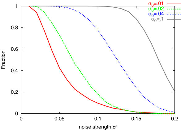
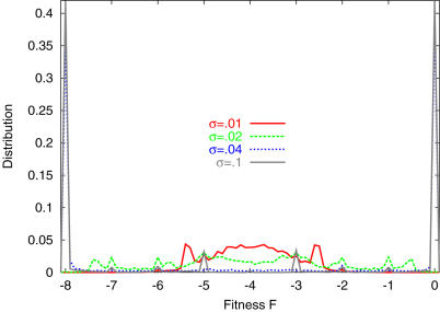
Phenotype of biological systems needs to be robust against mutation in order to sustain themselves between generations. On the other hand, phenotype of an individual also needs to be robust against fluctuations of both internal and external origins that are encountered during growth and development. Is there a relationship between these two types of robustness, one during a single generation and the other during evolution? Could stochasticity in gene expression have any relevance to the evolution of these types of robustness? Robustness can be defined by the sharpness of the distribution of phenotype; the variance of phenotype distribution due to genetic variation gives a measure of 'genetic robustness', while that of isogenic individuals gives a measure of 'developmental robustness'. Through simulations of a simple stochastic gene expression network that undergoes mutation and selection, we show that in order for the network to acquire both types of robustness, the phenotypic variance induced by mutations must be smaller than that observed in an isogenic population. As the latter originates from noise in gene expression, this signifies that the genetic robustness evolves only when the noise strength in gene expression is larger than some threshold. In such a case, the two variances decrease throughout the evolutionary time course, indicating increase in robustness. The results reveal how noise that cells encounter during growth and development shapes networks' robustness to stochasticity in gene expression, which in turn shapes networks' robustness to mutation. The necessary condition for evolution of robustness, as well as the relationship between genetic and developmental robustness, is derived quantitatively through the variance of phenotypic fluctuations, which are directly measurable experimentally.

Figure 1. Evolutionary time course of the fitness F̅.

The highest (a) and the lowest (b) values of the fitness F̅ among all individuals that have different genotypes (i,e., networks J_ij) at each generation are plotted. Plotted are for different values of noise strength, σ = 0.01,0.02,0.04,0.06,0.08,0.1, 0.2 with different color. Hereafter we mainly present the numerical results for M = 64 and k = 8. At each generation there are N individuals. N_s = N/4 networks with higher values of F̅ are selected for the next generation, from which mutants with a change in a single element J_ij are generated. For the average of fitness, L runs are carried out for each. Unless otherwise mentioned, we choose N = L = 300, while the conclusion to be shown does not change as long as they are sufficiently large. (We have also carried out the selection process by F instead of F̅, but the conclusion is not altered if N is chosen to be sufficiently large.) Throughout the paper, we use β = 7.

Figure 2. Average fitness <F̅>, lowest average fitness F̅ _min, evolution speed, and variance of the fitness V_g are plotted against the noise strength σ.

<F̅>, the average of the average fitness F̅ over all individuals is computed for 100–200 generations (red cross, from the simulation with population of 100 individuals, and purple square from 300 individuals). The minimal fitness is computed from the time average of the least fit network present at each generation (green, from 100 population, and light blue from 300). The evolution speed is plotted, measured as the inverse of the time required for the top individual to reach the maximal fitness 0. V_g is computed as the variance of the distribution P(F̅) at 200th generation.

Figure 3. Distribution P(F̅) after 200 generations, for population of 1000 individuals.

Inset is the magnification for −0.2<F̅<0. For high σ (red, with σ = 0.1), the distribution is concentrated at F̅ = 0, while for low σ (green, with σ = 0.006), the distribution is extended to large negative values, even after a large number of generations.

Figure 4. Relationship between V_g and V_ip. V_g is computed from P(F̅) at each generation, and V_ip by averaging the variance of p(F; gene) over all existing individuals.

(We also checked by using the variance for such gene network that gives the peak fitness value in P(F̅), but the overall relationship is not altered). Plotted points are over 200 generations. For σ>σ_c≈.02, both decrease with generations.

Figure 5. Dependence of the fraction of the runs that reach the target expression pattern. Networks that had the top fitness value under noise σ were simulated at a different noise σ′.

We first generate a network as a result of evolution over 200 generations under the noise strength σ, and select such network J_ij that has the top fitness value. Then we simulate this network under new noise strength σ′ from the initial condition −1,−1,…,−1 over 10000 runs, to check how many of them reach the target pattern (i.e., x_i>0 for i = 1 to 8). Plotted is the fraction of such runs against the noise strength σ′. Different color corresponds to the value of the original noise strength σ used for the evolution of the network.

Figure 6. Distribution of the fitness value when the initial condition for x_j is not fixed at −1, but is distributed over [−1,1]

. We choose the evolved network as in Fig. 5, and for each network we take 10000 initial conditions, and simulated the dynamics (1) without noise to measure the fitness value F after the system reached an attractor (as the temporal average 400<t<500). The histogram is plotted with a bin size 0.1.

Figure 7. Schematic representation of the basin structure, represented as a process of climbing down a potential landscape.

Δ is the magnitude of perturbation to jump over the barrier to a different attractor from the target. Smooth landscape is evolved under high level noise (above), and rugged landscape is evolved under low level noise (below).

Figure 8. Schematic representation of an orbit in the phase space.

The solid curve is an original orbit from the initial condition (I) to the target attractor (T). Dashed curves are orbits perturbed by noise. When orbits encounter turning points, they escape the original basin of attraction and may be caught in another attractor. Mutations, on the other hand, are able to move the position of turning points.

References

-
- Barkai N, Leibler S. Robustness in simple biochemical networks. Nature. 1997:913–917. - PubMed
- Alon U, Surette MG, Barkai N, Leibler S. Robustness in bacterial chemotaxis, Nature. 1999:168–171. - PubMed
- Wagner A. Robustness against mutations in genetic networks of yeast. Nature Genetics, 2000:355–361. - PubMed
- de Visser JAGM, et al. Evolution and detection of genetic robustness. Evolution. 2003:1959–1972. - PubMed
MeSH terms
LinkOut - more resources
Full Text Sources
Research Materials