Automation of random conical tilt and orthogonal tilt data collection using feature-based correlation

Abstract

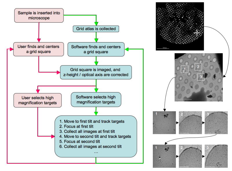
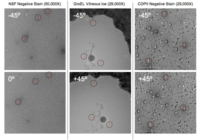
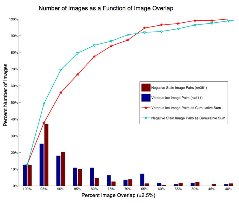
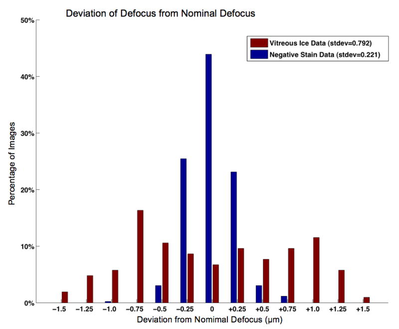
Visualization by electron microscopy has provided many insights into the composition, quaternary structure, and mechanism of macromolecular assemblies. By preserving samples in stain or vitreous ice it is possible to image them as discrete particles, and from these images generate three-dimensional structures. This 'single-particle' approach suffers from two major shortcomings; it requires an initial model to reconstitute 2D data into a 3D volume, and it often fails when faced with conformational variability. Random conical tilt (RCT) and orthogonal tilt (OTR) are methods developed to overcome these problems, but the data collection required, particularly for vitreous ice specimens, is difficult and tedious. In this paper, we present an automated approach to RCT/OTR data collection that removes the burden of manual collection and offers higher quality and throughput than is otherwise possible. We show example datasets collected under stain and cryo conditions and provide statistics related to the efficiency and robustness of the process. Furthermore, we describe the new algorithms that make this method possible, which include new calibrations, improved targeting and feature-based tracking.

Figure 1

An overview of automated RCT/OTR data collection as experienced by the end user. The boxes in red depict actions a user must perform while the boxes in blue depict functions performed by Leginon. The red arrows denote the semi-automated approach where a user must select the regions they are interested in imaging and the software handles the rest. The green arrows depict the fully automated approach where Leginon determines the regions of interest automatically. The images on the right provide a visual example of each step in the process and demonstrate the order in which images are collected.

Figure 2

The three panels illustrate the microscope z-height and optical axis alignment that is performed prior to automated collection of RCT or OTR data. Panel A shows the image translation (red arrow) seen when the microscope z-height is set incorrectly and the stage is tilted to either side of 0°. By measuring this displacement it is possible to correct the z-height regardless of the position of the optical axis. Panel B shows the microscope when the z-height is set correctly but the tilt axis is misaligned with the optical axis. This misalignment manifests itself, as shown, as another image displacement and defocus change when the stage is tilted away from 0°. Since this alignment has no effect when the stage remains at 0° it is commonly ignored in standard data collection. Fortunately it can be corrected electronically by using an image shift adjustment to compensate. Panel C shows the final aligned state where sample remains within a consistent focal plane regardless of tilt angle or stage movement (stage movements translate the specimen along the tilt plane).

Figure 3

Shown, is an overview of feature detection and matching. Panel A is a view of a grid square at 0° tilt. The border of a region (in this case a hole in the carbon) found using MSER is shown in red, and around it, in green, is the ellipse that has been fitted to the border (the ellipse radii are multiplied by 2). In the blue inset is the normalized feature (using the fitted ellipse parameters), on the left, and its derivative image, on the right. The green graph, superimposed in the panel, represents the PCA-SIFT descriptor for this feature, and is composed of the 36 principal components derived from the derivative image. Panel B shows two features found in an image of the same grid square tilted to 55°. Of note is that the fitted ellipses are now eccentric, and when normalized, the features become circular. This illustrates the reason why the MSER detector is affine invariant. The PCA-SIFT descriptors for two features in Panel B are also shown, and as expected, the feature that corresponds to the one in panel A has a very similar descriptor, while the other does not. The fact that the descriptors do not match perfectly has several potential sources, i.e. noise, detector instability, and the fact that an EM image is created by projection rather than reflection. Reasonable differences between correctly matched descriptors are fairly common in feature tracking, where the most important criterion is generally not how perfect a correct match is, but how well it compares to all the incorrect matches.

Figure 4

An example OTR image pair taken from the COPII vitreous ice dataset. In panel A is the first tilt image of a pair, taken at -45°, showing considerable charging towards the bottom half of the image. The charging resembles drift except that the effect is localized to only a portion of the image. In panel B is the second image (at 45°) taken 30 minutes later showing little evidence of the previous charging. The image overlap for this pair was ~90%. This image pair was taken before the use of a pre-exposure timing on the camera shutter.

Figure 5

Example tilt pairs taken from the NSF negative stain, GroEL in vitreous ice, and COPII in negative stain datasets, these images are representative of most images in the dataset. An example of the COPII dataset was shown in Figure 4. Landmarks have been highlighted to make the image overlap easier to assess by eye. The tilt axis in these images largely runs along the y axis, though there is a small rotational component of about 5-10° in the orientation of the tilt axis between each pair. This is an example of a difference that is automatically incorporated when using feature based tracking. Note that in comparison to the vitreous ice tilt pair shown in Figure 3, the GroEL (on CryoMesh™) image pair shows no sign of charging in either image even without the use of pre-exposure.

Figure 6

A histogram that plots the number of images (as a percent of the total number) vs. the percent image overlap between tilt pairs. For example, ~38% of the negative stain image pairs, and ~25% of the vitreous ice image pairs, have an overlap of 95% ± 2.5%. The line graphs represent the cumulative sum of these distributions and are included to aid in an alternate assessment of the image overlap. For example, ~80% of the vitreous ice image pairs have an overlap greater than, or equal to, 77% and ~80% of the negative stain image pairs have an overlap of greater than, or equal to, 85%.

Figure 7

A bar graph showing the deviation between the measured defocus and the nominal defocus for the image pairs collected. As can be seen the negative stain dataset is very tightly clustered around the desired defocus, while the ice datasets, are not as tightly clustered, but fall within a useable range of defocus values.

References

1. Brink J, Sherman MB, Berriman J, Chiu W. Evaluation of charging on macromolecules in electron cryomicroscopy. Ultramicroscopy. 1998;72:41–52. - PubMed
1. Brown M, Lowe D. Automatic Panoramic Image Stitching Using Invariant Features. International Journal of Computer Vision 2006
1. Fischler MA, Bolles RC. Random Sample Consensus - a Paradigm for Model-Fitting with Applications to Image-Analysis and Automated Cartography. Communications of the Acm. 1981;24:381–395.
1. Fitzgibbon A, Pilu M, Fisher RB. Direct least square fitting of ellipses. Ieee Transactions on Pattern Analysis and Machine Intelligence. 1999;21:476–480.
1. Frank J. Three-dimensional electron microscopy of macromolecular assemblies : visualization of biological molecules in their native state. 2. Oxford University Press; New York: 2006.
Publication types
MeSH terms
LinkOut - more resources