The effect of temperature and thermal acclimation on the sustainable performance of swimming scup

Abstract

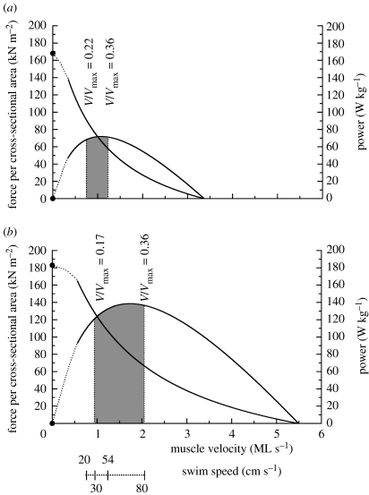
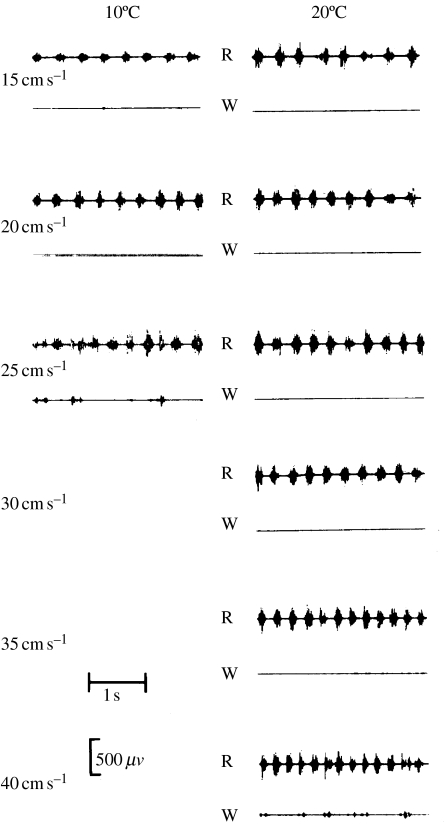
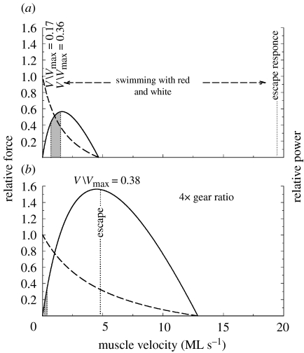
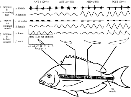
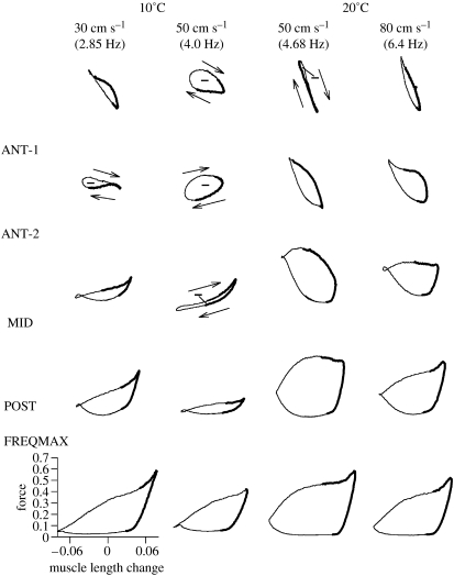
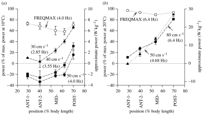
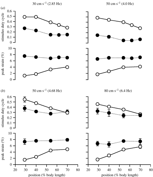
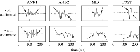
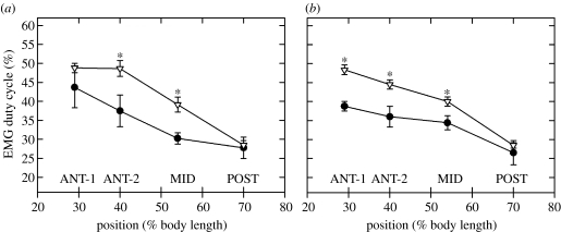
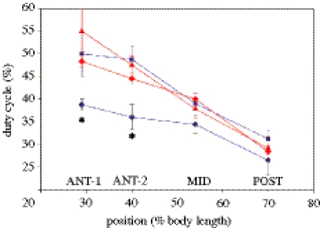
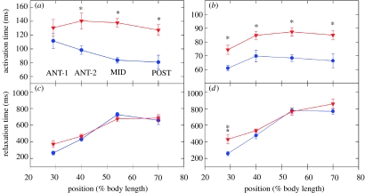
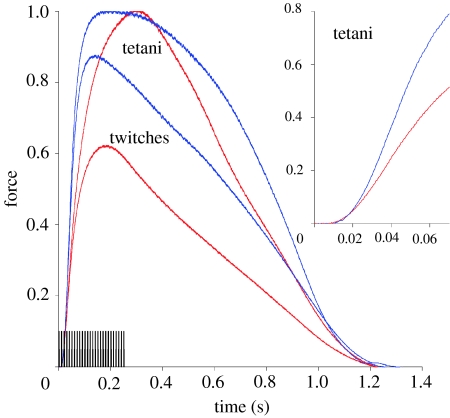
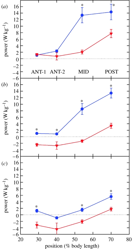
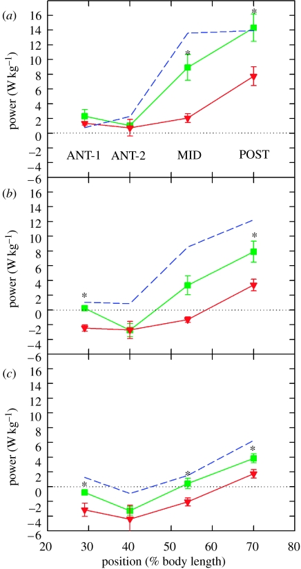
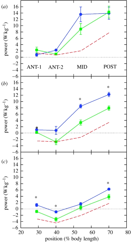
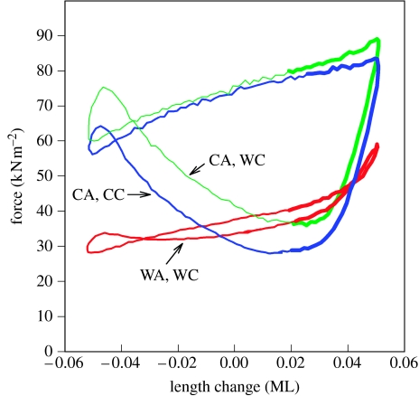
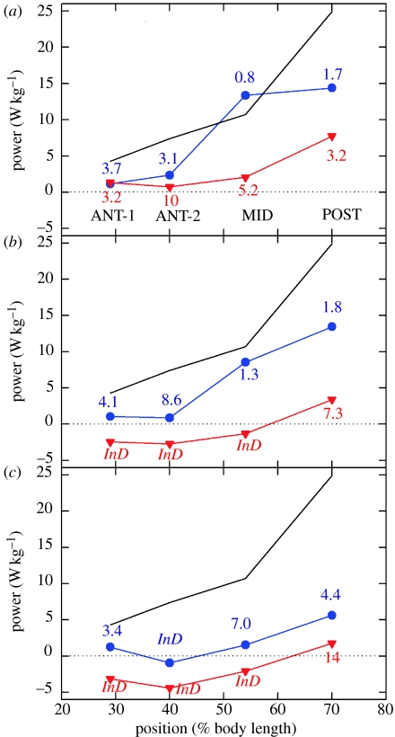
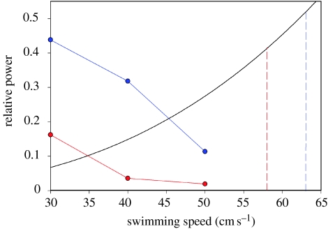
There is a significant reduction in overall maximum power output of muscle at low temperatures due to reduced steady-state (i.e. maximum activation) power-generating capabilities of muscle. However, during cyclical locomotion, a further reduction in power is due to the interplay between non-steady-state contractile properties of muscle (i.e. rates of activation and relaxation) and the stimulation and the length-change pattern muscle undergoes in vivo. In particular, even though the relaxation rate of scup red muscle is slowed greatly at cold temperatures (10 degrees C), warm-acclimated scup swim with the same stimulus duty cycles at cold as they do at warm temperature, not affording slow-relaxing muscle any additional time to relax. Hence, at 10 degrees C, red muscle generates extremely low or negative work in most parts of the body, at all but the slowest swimming speeds. Do scup shorten their stimulation duration and increase muscle relaxation rate during cold acclimation? At 10 degrees C, electromyography (EMG) duty cycles were 18% shorter in cold-acclimated scup than in warm-acclimated scup. But contrary to the expectations, the red muscle did not have a faster relaxation rate, rather, cold-acclimated muscle had an approximately 50% faster activation rate. By driving cold- and warm-acclimated muscle through cold- and warm-acclimated conditions, we found a very large increase in red muscle power during swimming at 10 degrees C. As expected, reducing stimulation duration markedly increased power output. However, the increased rate of activation alone produced an even greater effect. Hence, to fully understand thermal acclimation, it is necessary to examine the whole system under realistic physiological conditions.

Figure 1

Influence of temperature on mechanical properties of scup red muscle and on their use during swimming. This figure shows the average (see note below) force–velocity and power–velocity curves of scup red muscle at (a) 10°C and (b) 20°C. (NB the dotted portion of the curves were not covered by their experiments and are fit by eye based on previous results). As muscle-shortening velocity during steady swimming was independent of temperature, we have placed the swimming speed axis on the graph as well. Thus, during steady swimming, the curves provide the power, force and muscle-shortening velocity as a function of swimming speed. The shaded regions represent the muscle-shortening velocity during steady swimming with red muscle. The dotted vertical lines at each temperature represent transition swimming speeds (see Rome et al. 1990). At slower swimming speeds than that of the left-most line, the scup used ‘burst and coast’ swimming with red muscle or their pelvic fins. At higher swimming speeds than that of the right-most line, the white muscle is recruited and the scup used burst-and-coast swimming. For each temperature, the V/V_max at the transition points is given. Adapted from Rome et al. (1992b).

Figure 2

(a) Sarcomere length excursion, (b) tail-beat frequency, (c) muscle velocity, (d) tail-beat amplitude and (e) tail height as a function of swimming speed at 10°C (filled circle) and 20°C (open triangle) in the posterior position of the fish. The influence of swimming speed on sarcomere length excursion was small and temperature had no effect. Temperature had no effect on tail-beat frequency but there was a linear increase of tail-beat frequency with swimming speed at the two temperatures. Muscle velocities increase linearly with swimming speed due to the increase in tail-beat frequency. Temperature generally had no effect on velocities. Neither swimming speed nor temperature had an influence on tail-beat amplitude or tail height.

Figure 3

Electrical activity of red and white muscles during swimming at different speeds and temperatures in carp. At both temperatures, the carp recruited only the red muscle at low speeds and white muscle at higher speeds where the fish fatigued quickly. Hence, the same recruitment order was observed at both the temperatures; it was just compressed into a narrower speed range at 10°C.

Figure 4

Theorized recruitment of motor units as a function of swimming speed at (a) 10°C and (b) 20°C. Aerobic fibres, shaded motor units 1–3; anaerobic fibres, unshaded motor units 4–10. This schematically illustrates the compression of the recruitment order, and that all the aerobic fibres are recruited at a lower speed at 10°C, thus causing recruitment of the white muscle and rapid fatigue. Adapted from Rome (1990).

Figure 5

(a) Relative force, (b) power, (c) rate of energy usage and (d) efficiency as a function of relative shortening velocity for cold and warm muscles. Curves are shown for a cold fibre (solid) and a warm fibre (dashed). Respective V_max values are shown on the velocity axis. V₁ and V₂ are arbitrarily chosen examples for low and high velocities. Adapted from Rome (1990).

Figure 6

V/V_max in swimming carp. Force–velocity and power–velocity curves of the (a) red muscle and (b) white muscle. During steady swimming, the red muscle shortens at a velocity of 0.7–1.5 muscle lengths (ML) s⁻¹ (shaded region) corresponding to a V/V_max of 0.17–0.38 where maximum power and efficiency are generated. The red fibres cannot power the escape response because they would have to shorten at 20 ML s⁻¹ (a) or four times their V_max. The escape response is powered by the white muscle which, owing to its four-times-higher gear ratio, need shorten at only 5 ML s⁻¹, which corresponds to a V/V_max=0.38 where maximum power is generated (b). The white muscle would not be well suited to power steady swimming movements (shaded, b), as it would have to shorten at a V/V_max of 0.01–0.03, where power and efficiency are low. Adapted from Rome et al. (1988).

Figure 7

(a) Net power output at 10°C (open circles) and 20°C (filled circles) and (b) Q₁₀ for power output as a function of oscillation frequency. Note that the appropriate swimming speed (from Rome et al. 1992a) for each oscillation frequency over which the scup use their red muscle is shown. Adapted from Rome & Swank (1992).

Figure 8

EMG duty cycle as a function of tail-beat frequency (swimming speed) at 10°C (red filled circles) and 20°C (black filled circles). Note that there is no difference in duty cycle at 10 and 20°C, but that as swimming speed increases, EMG duty cycle declines. Note also that the swimming speed scale differs slightly from that in figure 7, as this scale was calculated for this particular fish. For comparison purposes, the stimulation duty cycles that we found produced optimal power output in the isolated muscle experiments are shown with dotted lines (red, 10°C; black, 20°C). Adapted from Rome & Swank (1992).

Figure 9

Length changes, stimulation pattern, force production and work output of red muscle during swimming. Step 1 was to measure in a swimming (80 cm s⁻¹) fish the (a) EMGs and (b) length changes for the red muscle at four places along the length of the fish pictured. Step 2 was to impose on muscle bundles isolated from these four positions the (d) length changes and (c) stimulation pattern that were observed during swimming. Step 3 was to measure in the isolated muscle the resulting (e) force production and (f) work production. Traces a to e are all functions of time. Trace f is a plot of force produced against length changes where the area of the enclosed loop is the work produced during a tail-beat cycle. This value is much larger in the POST than in the ANT-1 position. Adapted from Rome et al. (1993).

Figure 10

Representative work loops for all in vivo conditions. The first four rows of each column show the work loops generated by a red muscle bundle from each position when driven under four sets of in vivo conditions (as measured in Swank & Rome 2000). The 80 cm s⁻¹ data at 20°C are from Rome et al. (1993). The bottom row (FREQMAX) shows work loops generated when muscle length change, stimulus duration and phase were optimized to generate maximum power at the stated in vivo oscillation frequency and temperature. The timing of the stimulus relative to the total length-change cycle is represented by the thickening of the loop. Loops denoted by a negative sign generated net negative work and progress in a clockwise direction, whereas unmarked loops generated net positive work and progressed in the clockwise direction. Force was normalized to isometric force at 20°C. The x- and y-axes in the bottom left-hand graph represent scale bars for all the work loops. The muscle used for the bottom row (FREQMAX) was an ANT-1 bundle. This muscle was driven at the same frequency as the muscles above it, but the stimulation and length-change conditions were optimized for that frequency. Hence, the low work output at 10°C is not due to an inability of the muscle to generate power, but due to the in vivo conditions. Adapted from Rome et al. (2000).

Figure 11

In vivo power generated by muscle bundles from different positions along the fish at different swimming speeds and temperatures. (a) 10°C and (b) 20°C. Note that power is extremely dependent on position and is generally far smaller than the maximum power that the muscle could generate at the stated in vivo oscillation frequency (FREQMAX) except in the POST position at certain speeds. Power is expressed as a percentage of the maximum power-generating ability of the muscle at the experimental temperature (left y-axis). The right y-axis shows the approximate absolute power generated by the muscles expressed in W kg⁻¹ (note the difference in scale at 10°C when compared with 20°C). Note also that the absolute power scale is only approximate because values at each temperature are normalized for maximum power averaged over all the positions. Data at 80 cm s⁻¹ at 20°C are from Rome et al. (1993). Adapted from Rome et al. (2000).

Figure 12

Comparison of stimulus duty cycle and strain values that maximize power (‘optimized’; filled symbols, dotted lines) with values measured in vivo (open symbols, solid lines) at (a) 10°C and (b) 20°C. The difference was greatest at the anterior positions and at 10°C. In addition, at 10°C, increased swimming speed led to a greater difference between optimal and in vivo conditions (t-test on difference of means, p<0.001). Results from manual analysis of EMG duration (circles) are shown for all temperatures and speeds.

Figure 13

Cross-section of the scup myotomal muscle at the ANT-2 position stained with myosin ATPase (alkali pre-incubation, pH 10.2). Pink fibres are stained dark, unstained small fibres are red muscle fibres and unstained large fibres are white muscle fibres. The red, pink and white muscle layers are labelled r, p and w. The lateral margin of the fish is up, and dorsal is to the left. Scale bar is 1.0 mm. The circle represents the region from which muscle bundles of relatively pure pink fibre content were extracted. Adapted from Coughlin et al. (1996).

Figure 14

(a) Schematic of the scup showing the location of the steaks that were cut from the fish (S1–S8; dotted boundaries). ΔL, thickness of the segments (see text). Hatching refers to where the steak was sectioned. (b) The cross-sections of steaks from the anterior (ANT-2), middle and posterior position of the fish, showing the locations of each fibre type (R, red; P, pink; W, white). Adapted from Zhang et al. (1996).

Figure 15

(a) Tetanus and (b) twitch records at 20°C for red- and pink-muscle bundles. Individual traces were normalized to the peak force of that contraction. For each record, the stimulus (either a repeated train of pulses for tetanus or a single pulse for twitch stimulation) was optimized such that the muscle bundle generated maximum force. Stimulation began at time zero. (a) The stimulation duration of the tetanus is represented by the thickening of the force trace. Since pink muscle do not maintain steady tetanic force as long as red-muscle, tetanus stimulation duration was limited and the broad plateau observed for the red-muscle tetanus record is not observed in pink-muscle tetanus records.

Figure 16

Work loops from red and pink muscle when run under in vivo conditions at 10°C. Red- and pink-muscle bundles were activated with their respective in vivo length change and stimulation pattern. Area of the loop signifies work per cycle. As all cycles are at the same frequency, the 4.0 Hz tail-beat frequency for swimming at 50 cm s⁻¹, the area of the loop also indicates relative power generation. The work loops for the red muscle at ANT-1, ANT-2 and MID positions are primarily clockwise signifying that negative work is being produced. For the red muscle at the POST position and all the pink muscle, the loops are anticlockwise signifying positive work is being produced. Adapted from Coughlin & Rome (1996).

Figure 17

Comparison of total power generated by scup red and pink musculature at the maximum sustainable swimming speeds at (a) 20°C (80 cm s⁻¹) and (b) 10°C (50 cm s⁻¹). The height of each bar of the histogram corresponds to the power that the red (black shading) and pink (grey shading) musculature generates at that location (i.e. the product of muscle mass and mass-specific power production). Pink muscle data are from Coughlin & Rome (1996). Note that these pink-muscle measurements were made on bundles taken exclusively from the ANT-2 position because it is not possible to obtain pure pink-muscle bundles from other positions. Note also that the in vivo conditions for the POST position were approximated as those of the red muscle at this position because there was not sufficient pink muscle at the POST from which to record EMGs. (c) The relative cross-section of the red (black circles) and pink muscle (grey circles) along the length of the fish (data from Zhang et al. 1996).

Figure 18

EMG traces from the four longitudinal electrode positions showing the longer EMG duration of warm-acclimated when compared with cold-acclimated scup red muscle. The start times of the ANT-1 bursts were used to align the traces. Both fish were swum at 50 cm s⁻¹ in 10°C water. Arrows mark start and stop times of the EMGs determined manually. Adapted from Rome & Swank (2001).

Figure 19

EMG duty cycle for cold- and warm-acclimated scup swimming at (a) 30 cm s⁻¹ and (b) 50 cm s⁻¹ in 10°C water. Duty cycle was EMG duration divided by tail-beat frequency and was significantly shorter in the cold-acclimated scup. Asterisk, significant difference at a given body position due to acclimation; filled circles, cold acclimated; inverted open triangles, warm acclimated. Adapted from Rome & Swank (2001).

Figure 20

Stimulus duty cycle under the four acclimation-temperature and acute-temperature conditions. For the warm-acclimated 10°C (red, filled diamond) and 20°C (red, filled triangle) swimming conditions and the cold-acclimated 20°C (blue, filled square) swimming conditions, the stimulus duty cycles were nearly the same (there was no statistical difference). There was however a significant reduction in duty cycle in the cold-acclimated 10°C (blue, filled circle) swimming conditions (significant at ANT-1 and ANT-2 but not significant at POST). Asterisk, significant reduction. Adapted from Rome & Swank (2001).

Figure 21

(a) Tetanic activation time and (c) tetanic relaxation time (T_r,90-10) of cold- and warm-acclimated scup red muscle. Activation time was statistically significant due to acclimation (asterisk). Relaxation differences due to acclimation were not statistically significant. Similar differences between the acclimation groups (b, activation time and d, relaxation time) were obtained from twitches as well. Red filled inverted triangle, warm acclimated scup; blue filled circle, cold acclimated scup. Adapted from Swank & Rome (2001).

Figure 22

Isometric twitches and tetani from warm- (red) and cold-acclimated (blue) scup red muscle under identical conditions. Bundles are from the MID position. Stimulus duration for the tetanus is 250 ms. Force levels were normalized to maximum isometric force of each muscle. Note the longer time to reach maximum force and lower twitch tetanus ratio in the warm-acclimated muscle. Inset: force records for tetani shown with a faster time base. Adapted from Swank & Rome (2001).

Figure 23

In vivo power from scup red muscle. Muscle bundles from cold-acclimated scup were driven through cold-acclimated in vivo conditions at 10°C and muscle from warm-acclimated scup was driven through warm-acclimated in vivo conditions at 10°C. The swimming speeds were (a) 30 cm s⁻¹ (2.85 Hz), (b) 40 cm s⁻¹ (3.5 Hz) and (c) 50 cm s⁻¹(4.0 Hz). Power differences due to acclimation at all swimming speeds were statistically significant. Asterisk, significant difference due to acclimation at individual position; blue filled circle, cold-acclimated muscle and cold-acclimated conditions; red filled inverted triangle, warm-acclimated muscle and warm-acclimated conditions. Error bars are one standard error. Adapted from Swank & Rome (2001).

Figure 24

Increased power due to acclimation-induced changes in red-muscle mechanical properties. In these experiments, warm- and cold-acclimated bundles were run under the same warm-acclimated in vivo conditions. The swimming speeds were (a) 30 cm s⁻¹, (b) 40 cm s⁻¹ and (c) 50 cm s⁻¹. Power differences due to muscle acclimation at all swimming speeds were statistically significant. Asterisk, significant difference due to acclimation at individual positions; blue dashed lines, cold-acclimated muscle and cold-acclimated conditions; green filled square, cold acclimated muscle and warm acclimated conditions; red filled inverted triangle, warm-acclimated muscle and warm-acclimated conditions. For comparison to the total change in power output associated with cold acclimation, power output of the cold-acclimated muscle running under cold-acclimated conditions is shown as a dashed blue line. Adapted from Swank & Rome (2001).

Figure 25

Increased power due to acclimation-induced changes in in vivo conditions (primarily EMG duty cycle). In these experiments, cold-acclimated red muscle was run under both cold- and warm-acclimated in vivo conditions. The swimming speeds were (a) 30 cm s⁻¹, (b) 40 cm s⁻¹ and (c) 50 cm s⁻¹. This comparison shows the contribution of changes in the nervous system output to the increase in power production in cold-acclimated fish. Asterisk, significant difference due to different in vivo acclimation conditions at individual positions; blue filled circle, cold-acclimated muscle and cold-acclimated conditions; green filled square, cold-acclimated muscle and warm-acclimated conditions. For comparison with the total change in power output associated with cold acclimation, power output of the warm-acclimated muscle running under warm-acclimated conditions is shown as a dashed red line. Adapted from Swank & Rome (2001).

Figure 26

Power generated by warm- and cold-acclimated muscle. The two muscle bundles are from the POST position of warm-acclimated (WA) and cold-acclimated (CA) scup and were driven through POST in vivo conditions for a 40 cm s⁻¹ swimming speed. The warm-acclimated conditions (WC) were 3.6 Hz, 5.4% strain, −54° phase and 85 ms stimulus duration. Cold-acclimated conditions (CC) were 3.5 Hz, 5.4% strain, −56° phase and 80 ms stimulus duration. Power generation for WA, WC (red) was 1.4 W kg⁻¹; 9.1 W kg⁻¹ for CA, WC (green); and 12.6 W kg⁻¹ for CA, CC (blue). Note that for this particular swimming speed and anatomical position, there is only a small change in stimulus duty cycle and thus there is only a moderate enhancement in work production associated with the cold-acclimated conditions. Adapted from Swank & Rome (2001).

Figure 27

The temperature dependence of power output during swimming. Muscle power output at (a) 30 cm s⁻¹ (2.85 Hz), (b) 40 cm s⁻¹ (3.5 Hz) and (c) 50 cm s⁻¹ (4.0 Hz) and 10°C in cold-acclimated fish (blue) and warm-acclimated fish (red) are compared with power output during swimming at 80 cm s⁻¹ and 20°C in warm-acclimated fish (black line; data from Rome et al. 2000). Q₁₀ values (power at 20°C/power at 10°C) are given in the appropriate colour for each position and swimming speed. InD signifies that the Q₁₀ is indeterminate, i.e. the power output at 10°C is negative. Adapted from Swank & Rome (2001).

Figure 28

The relative total power output of the red musculature as a function of swimming speed at 10°C. The blue curve represents power output of the red musculature from cold-acclimated fish and the red curve represents power output from warm-acclimated fish. Relative power output of the red musculature was determined by integrating the power output of the red muscle along the length of the fish, and then normalizing to the integrated power output of the red+pink muscle of fish swimming at 80 cm s⁻¹ and 20°C (as outlined in Rome et al. 2000). We chose power output at 80 cm s⁻¹ and 20°C as an estimate of the maximum power output that the combined red and pink musculature can generate during swimming. This seems reasonable because 80 cm s⁻¹ is close to the swimming speed of initial white-muscle recruitment at 20°C, and we know that both pink and red muscle are recruited at this swimming speed (Coughlin & Rome 1999). The relative power required for swimming at slower speeds (black curve) was calculated based on the assumption that power required is proportional to the cube of swimming speed (Webb 1978): relative power required is proportional to (speed/80)³. This figure shows that there is a very large increase in total red-muscle power output associated with thermal acclimation, which probably permits the cold-acclimated fish to swim at 40 cm s⁻¹ with the red muscle alone, whereas the warm-acclimated fish cannot. However, at swimming speeds of 58–63 cm s⁻¹, the red musculature generates very little power and only a small proportion of the total power required to swim at that speed. Adapted from Swank & Rome (2001). Red dashed line, warm-acclimated white muscle recruitment speed (58 cm s⁻¹); blue-dashed line, cold-acclimated recruitment speed (63 cm s⁻¹).

References

1. Altringham J.D, Johnston I.A. Modelling muscle power output in a swimming fish. J. Exp. Biol. 1990;148:395–402.
1. Altringham J.D, Wardle C.S, Smith C.I. Myotomal muscle function at different locations in the body of a swimming fish. J. Exp. Biol. 1993;182:191–206.
1. Anderson E.J, McGillis W.R, Grosenbaugh M.A. The boundary layer of swimming fish. J. Exp. Biol. 2001;204:81–102. - PubMed
1. Beddow T.A, van Leeuwen J.L, Johnston I.A. Swimming kinematics of fast starts are altered by temperature acclimation in the marine fish Myoxocephalus scorpius. J. Exp. Biol. 1995;198:203–208. - PubMed
1. Bennett A.F. The thermal dependence of locomotor capacity. Am. J. Physiol. 1990;259:R253–R258. - PubMed
Publication types