From morphology to neural information: the electric sense of the skate

Abstract

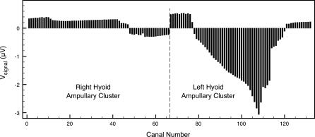
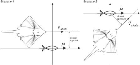
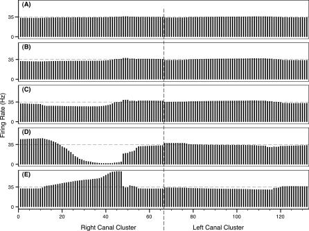
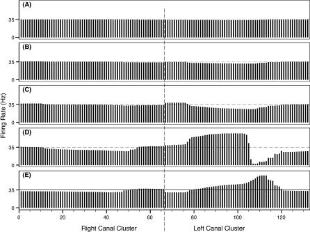
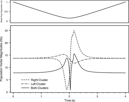
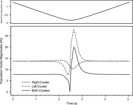
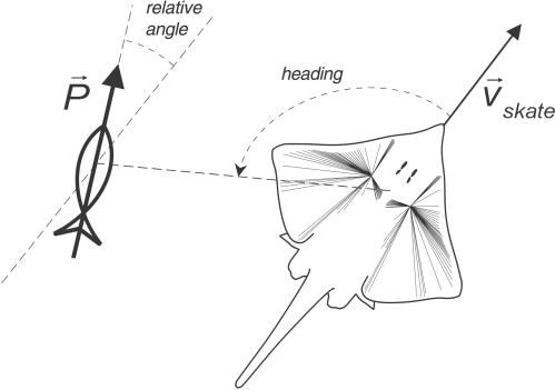
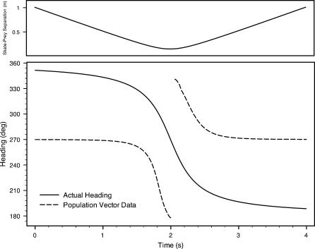
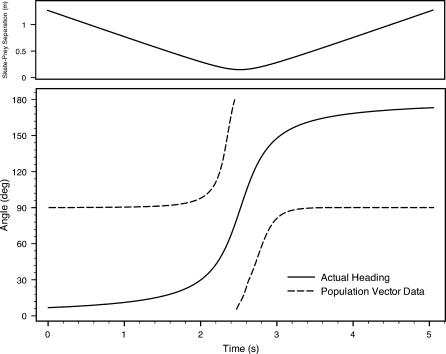
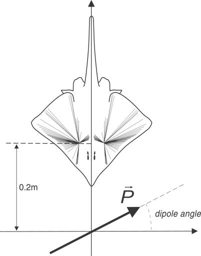
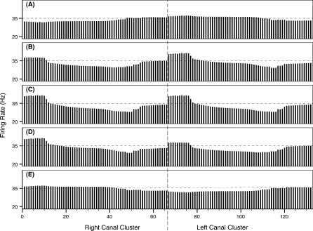
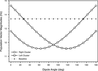
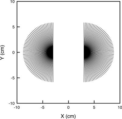
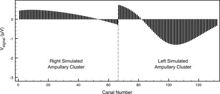
Morphology typically enhances the fidelity of sensory systems. Sharks, skates, and rays have a well-developed electrosense that presents strikingly unique morphologies. Here, we model the dynamics of the peripheral electrosensory system of the skate, a dorsally flattened batoid, moving near an electric dipole source (e.g., a prey organism). We compute the coincident electric signals that develop across an array of the skate's electrosensors, using electrodynamics married to precise morphological measurements of sensor location, infrastructure, and vector projection. Our results demonstrate that skate morphology enhances electrosensory information. Not only could the skate locate prey using a simple population vector algorithm, but its morphology also specifically leads to quick shifts in firing rates that are well-suited to the demonstrated bandwidth of the electrosensory system. Finally, we propose electrophysiology trials to test the modeling scheme.

Figure 1. Simplified Schematic Depicting Two Ampullae within a Single Cluster, with Their Associated Canals and Pores

Points A and C denote two pores, leading via gel-filled canals to their respective ampullae. Points B and D denote the inner ampullae, referencing electric potentials on the apical sides of the respective sensory epithelia. Point E is a common reference for the basal sides of ampullae within the cluster. The model used here emphasizes the potential differences arising along the internal gel of the narrow canals as driving the apical potentials, which lead to excitation or inhibition based on their relation to the relatively constant basal potential at point E (see text).

Figure 2. Canal Projections from the Dorsal Hyoid Ampullae of Raja laevis

(A) Adapted from [14]. (B) As used in the present modeling work. Here, ampullary clusters are treated as a single point for simplicity. (B) also presents the canal numbering used in plots in this study. The 132 dorsal hyoid canals in the barndoor skate morphology are numbered consecutively, with canals 1 to 66 in the right cluster, and canals 67 to 132 in the left cluster. As seen in the figure, the first canal in each cluster is the one pointing in the most forward direction, 4° off the longitudinal axis. The other canals in each cluster are numbered consecutively, clockwise for the right cluster, and counterclockwise for the left cluster. Locations of pores and ampullae used in modeling match those in the actual fish (A). In terms of potential differences between an ampulla and a pore for a given canal (which is what our model emphasizes), the physics of electromagnetism tells us that the actual shape of the canals is immaterial. Thus, we simply represent them as straight lines.

Figure 3. Skate Moving in a Source's Frame of Reference

A point in the skate (a pore or an ampulla) is labeled by the vector r in the source's reference frame.

Figure 4. Firing Rate Gain Function Used for Computing Neural Activity in the Primary Afferent Fibers Associated with the Ampullae

Available experimental data [11] was fitted to the sigmoid function 1.6 + 62 / (1 + 0.9 × exp(V_signal/11.5)).

Figure 5. Relative Ampullary Electric Signal Snapshot for a Skate Approaching a Source that Is 30 cm to Its Left and 10 cm in Front of It

Canal numbers correspond to those shown in Figure 1.

Figure 6. Two “Swim-By” Scenarios Used in the Simulations

Figure 7. Firing Rate Snapshots, Representing the Instantaneous System Activity for Swim-By Scenario 1

Snapshots when skate–source distance was 0.50 m (A), 0.35 m (B), 0.25 m (C), the closest approach of 0.15 m (D), and 0.20 m after the closest approach (E). The abscissa refers to the canal numbers described in Figure 2. The ordinate refers to the firing rates associated with each ampulla. Dashed line indicates resting discharge rate.

Figure 8. Firing Rate Snapshots, Representing the Instantaneous System Activity for Swim-By Scenario 2

Snapshots when skate–source distance was 0.50 m (A), 0.35 m (B), 0.25 m (C), the closest approach of 0.15 m (D), and 0.20 m after the closest approach (E). The abscissa refers to the canal numbers described in Figure 2. The ordinate refers to the firing rates associated with each ampulla. Dashed line indicates resting discharge rate.

Figure 9. Population Vector Magnitudes and Skate–Source Separation Distance (Top Panel) for Scenario 1

Figure 10. Population Vector Magnitudes and Skate–Source Separation Distance (Top Panel) for Scenario 2

Figure 11. Angular Measures in the Skate–Source Geometry

To prevent multivaluedness issues, we define all angles in the usual mathematical convention (i.e., 0°−360° range, counterclockwise with respect to the skate's longitudinal axis).

Figure 12. Net Population Vector Heading Data and Actual Source Heading versus Time for Scenario 1

The top graph depicts the separation distance over time. For this plot, a constant phase of 90° was added to the population vector data (see text).

Figure 13. Net Population Vector Heading Data and Actual Source Heading versus Time for Scenario 2

The top graph depicts the separation distance over time. For this plot, a constant phase of 90° was subtracted from the population vector data (see text).

Figure 14. Geometric Arrangement for the Simulated Skate–Dipole Benchtop Experiment

Figure 15. Firing Rate Snapshots Representing the Instantaneous System Activity for the Simulated Benchtop Experiment of Figure 14

The external electric dipole angle is 0° (A), 45° (B), 90° (C), 135° (D), and 180° (E). The abscissa refers to the canal numbers described in Figure 2. The ordinate refers to the DON firing rates associated with each one of these canals.

Figure 16. Population Vector Magnitude as a Function of the External Dipole Angle, as Defined in Figure 14

The “baseline” curve represents the magnitude of the population vector in the absence of an electric dipole field.

Figure 17. An Artificial Array of Canals for a Hypothetical Dorsal Hyoid Cluster

Figure 18. Relative Ampullary Electric Signal Snapshot for the Artificial Array Approaching a Source that is 30 cm to Its Left and 10 cm in Front of It

References

1. Volman SF, Kunishi M. Comparative physiology of sound localization in four species of owls. Brain Behav Evol. 1990;36:196–215. - PubMed
1. Sturzl W, Kempter R, van Hemmen JL. Theory of arachnid prey localization. Phys Rev Lett. 2000;84:5668–5671. - PubMed
1. Franosch JM, Sobotka MC, Elepfandt A, van Hemmen JL. Minimal model of prey localization through the lateral-line system. Phys Rev Lett. 2003;91:158101. - PubMed
1. Zakon HH. The electroreceptive periphery. In: Bullock TH, Heiligenberg W, editors. Electroreception. New York: Wiley; 1986. pp. 103–156.
1. Nelson ME, MacIver M. Prey capture in the weakly electric fish Apteronotus albifrons: Sensory acquisition strategies and electrosensory consequences. J Exp Biol. 1999;202:1195–1203. - PubMed