Standing waves and traveling waves distinguish two circuits in visual cortex

Abstract

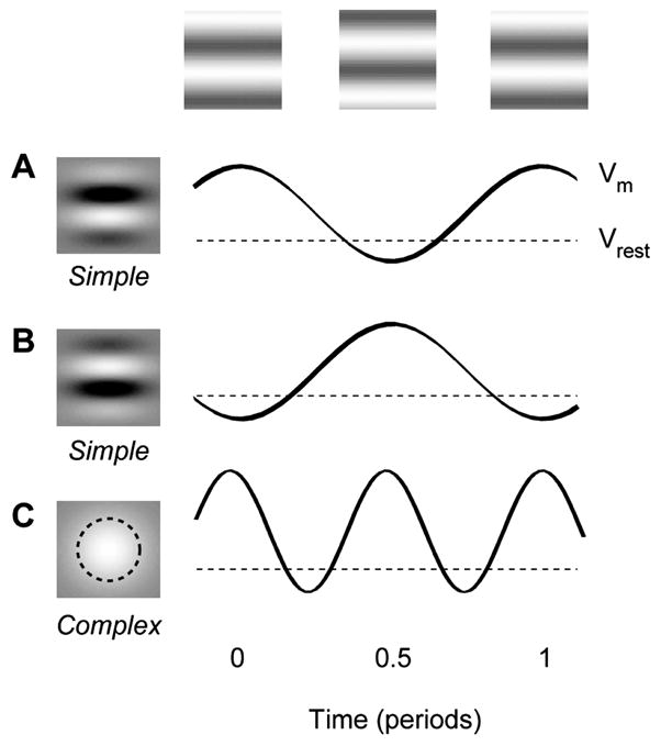
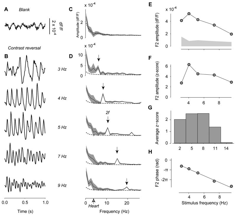
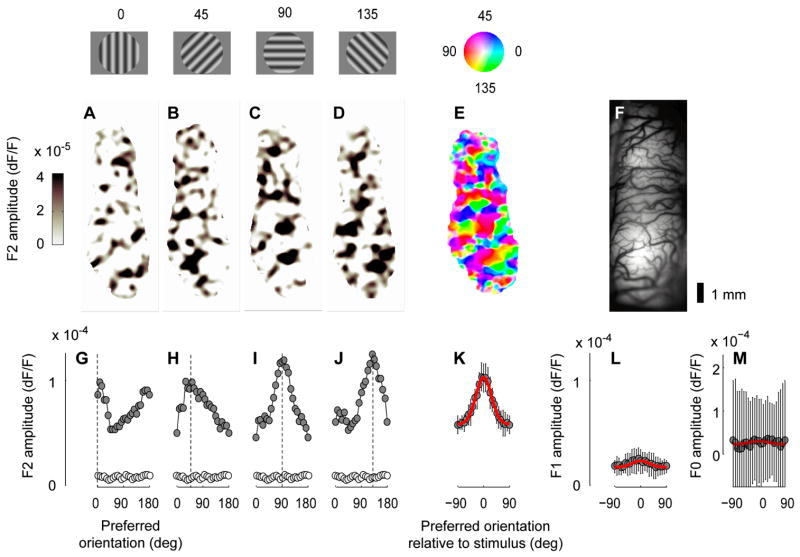
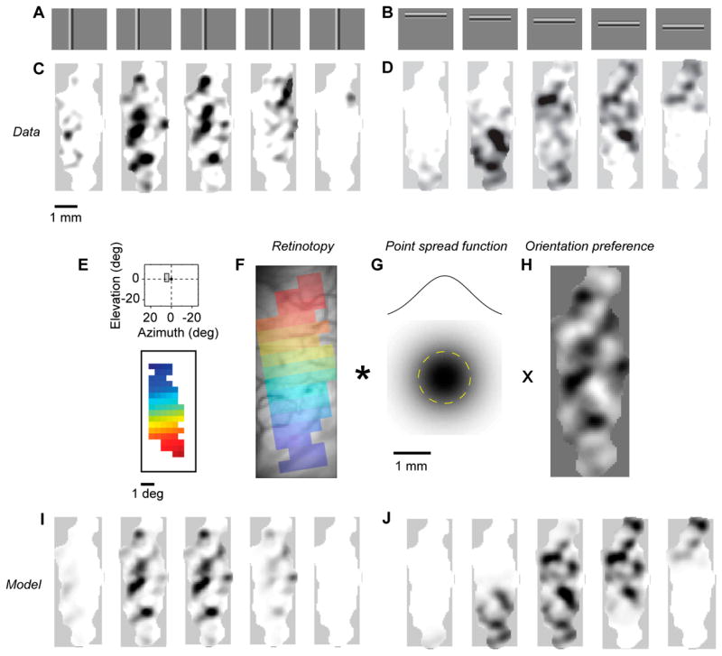
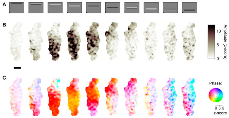
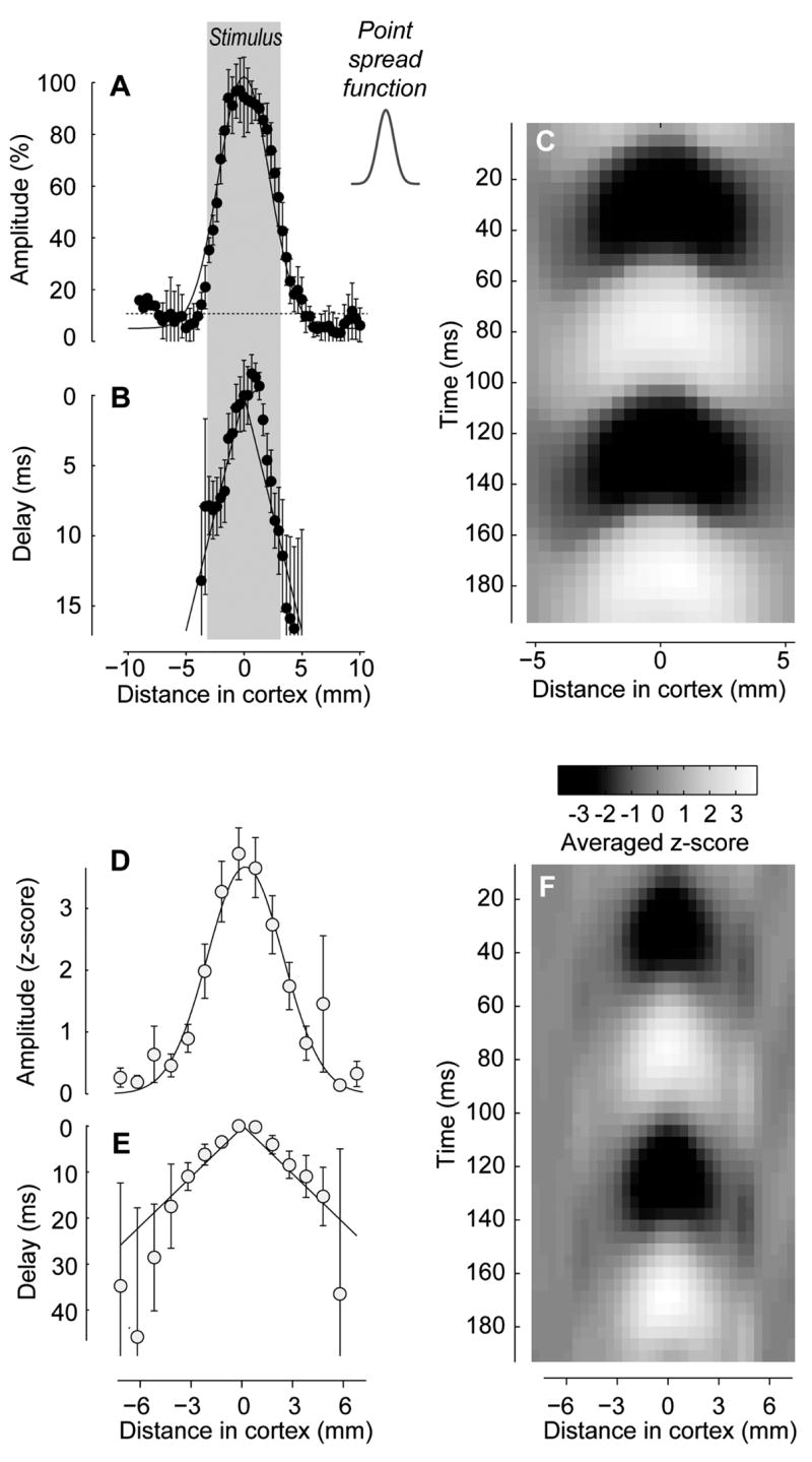
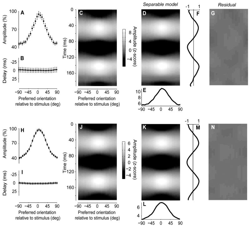
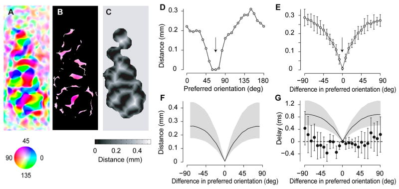
The visual cortex represents stimuli through the activity of neuronal populations. We measured the evolution of this activity in space and time by imaging voltage-sensitive dyes in cat area V1. Contrast-reversing stimuli elicit responses that oscillate at twice the stimulus frequency, indicating that signals originate mostly in complex cells. These responses stand clear of the noise, whose amplitude decreases as 1/frequency, and yield high-resolution maps of orientation preference and retinotopy. We first show how these maps are combined to yield the responses to focal, oriented stimuli. We then study the evolution of the oscillating activity in space and time. In the orientation domain, it is a standing wave. In the spatial domain, it is a traveling wave propagating at 0.2-0.5 m/s. These different dynamics indicate a fundamental distinction in the circuits underlying selectivity for position and orientation, two key stimulus attributes.

Figure 1

Responses of idealized simple and complex cells to a stimulus (a standing grating) whose contrast modulates sinusoidally in time. We illustrate the responses of three cells, whose receptive fields are shown in the left column. The dashed lines indicate the resting potential. (A) The membrane potential of a simple cell oscillates at the frequency of contrast reversal. (B) The oscillation will have the opposite sign in a second simple cell with a receptive field of opposite polarity. (C) The membrane potential of a complex cell oscillates at twice the frequency of the stimulus.

Figure 2

VSD responses to contrast-reversing stimuli, and basic properties of the 2^nd harmonic response. (A) VSD signals measured in response to a blank screen, averaged over 10.6 mm² of cortex. (B) VSD signals measured over the same area in response to a standing grating reversing in contrast at 3, 4, 5, 7, and 9 Hz. For graphical purposes, traces in A and B were high-pass filtered above 4 Hz. (C,D) Amplitude spectra of the responses in A,B. Gray traces show standard deviation measured by bootstrap over stimulus presentations (50 repeats). Dotted curve indicates 1/f^x fit to amplitude spectrum of the noise shown in A. Stimuli elicited strong responses at twice the frequency of contrast reversal (2^nd harmonic, arrows). (E) Amplitude of the 2^nd harmonic response as a function of stimulus frequency. The gray area indicates a measure of noise level, the average amplitude at the frequencies near (±2 Hz) the 2^nd harmonic. (F) Signal/noise ratios measured as z-scores (amplitude of the 2^nd harmonic divided by noise level). (G) Average across 5 experiments of the z-scores, as a function of stimulus frequency. (H) Phase of the 2^nd harmonic response as a function of stimulus frequency. The slope of the linear fit gives the integration time, 82 ms. Experiment 50-2-6.

Figure 3

Maps of orientation preference obtained from 2^nd harmonic responses. (AD) Amplitude of the 2^nd harmonic responses to standing gratings with different orientations, whose contrast reversed at 5 Hz. For graphical purposes, these maps were corrected by subtracting the average response to 8 orientations (“cocktail correction”), and ignoring negative responses. (E) Map of orientation selectivity obtained from these responses (plus other 4 that are not shown). Color indicates preferred orientation, and saturation indicates tuning amplitude (see pinwheel inset). (F) Reference image of the cortex illuminated with green light. (G–J) The population responses in A–D expressed as a function of pixel preferred orientation (obtained from the map in E). The open symbols indicate responses to a gray screen. (K) The population response expressed as a function of angle between preferred orientation and stimulus orientation, obtained by averaging the responses in G–J and those to 4 additional orientations. Error bars are s.d. computed over 8 stimulus orientations. A Gaussian fit is superimposed (curve). (L) Same, for the amplitude of the 1^st harmonic. (M) Same, for the mean of the responses (the 0^th harmonic). Experiment 50-2-3.

Figure 4

Maps of retinotopy obtained from 2^nd harmonic responses and their relation to the orientation preference maps. (A–B) Stimuli were gratings windowed in narrow rectangles. (C–D) Amplitude of 2^nd harmonic responses. The gray scale (white to black) spans the values between the 95^th and 99^th percentiles of the intensity distribution. (E–F) Map of retinotopy. The inset shows the region of visual field covered by the patch of cortex, in the same scale as the stimuli. (G) The point spread function estimated from data, which is modeled as a 2-D Gaussian. (H) Map of orientation preference (vertical minus horizontal). (I–J) Predictions of the model for the amplitude of 2^nd harmonic responses. Gray scale as in C–D. Experiments 67-2-1 and 67-2-2.

Figure 5

The oscillations in the 2^nd harmonic responses have different phases depending on stimulus position. (A) Stimuli are the same as Figure 4. (B) Amplitude of 2^nd harmonic responses (same data as in Figure 4D, only here it is shown in z-scores). (C) The phase of the 2^nd harmonic responses depends on distance from the stimulated region of cortex. Phase is coded by color according to pinwheel shown in the right, with color saturation varying with response amplitude. As indicated by the scale below the pinwheel, the phases of responses with z-scores below about 2 are shown in white. Color-coded phase varies smoothly from yellow in regions that are retinotopically centered on the stimulus to red, purple, and then cyan in regions that are progressively more distant. Experiment 67-2-1.

Figure 6

Traveling waves in the spatial domain. (A) Amplitude of the 2^nd harmonic responses shown in Figure 5B, expressed as a function of distance from the retinotopic location of the stimulus. This representation collapses the two dimensions of cortex into one, and combines the contributions of all stimuli. The curve is a Gaussian fitted to the data (σ = 2.2 mm). The horizontal line indicates the average noise level. The gray region indicates the extent of the retinotopic representation of the stimulus in cortex. The inset shows the estimated points spread function for this experiment (σ = 0.7 mm) (B) The phase of these averaged 2^nd harmonic responses, converted to delay in ms to facilitate the estimation of speed. The lines indicates the best linear fit (slope = 0.30 m/s). This fit was performed by imposing that the lines on each side of the origin have the same slope, and intercept at the origin at a value of zero. (C) The traveling wave in space-time. Activity is shown for one period of the stimulus (about 200 ms), averaged over periods and over repeats, and bandpass filtered at 7–13 Hz to emphasize the visually-driven responses. Gray levels go from −100% to 100%. (D–F) Same as A–C but averaged over 6 experiments. Gray levels indicate z-scores; they can be positive or negative, indicating standard deviations above or below the mean.

Figure 7

Standing waves in the orientation domain. (A) Amplitude of the 2^nd harmonic responses as a function of angle between the preferred orientation and the stimulus orientation (as in Figure 3K). (B) Phase of these 2^nd harmonic responses. (C) Space-time representation (as in Figure 6C, except that population responses are expressed as a function of preferred orientation rather than cortical distance). (D–F) The predictions of the best separable model, which is the product of a function of orientation in E and the time course in F. (G) The residual obtained by subtracting the model predictions in D from the responses in C. Experiment 50-2-3. (H–N) The same analysis, performed on the average of the responses in 23 experiments. Curve in H is a Gaussian fit.

Figure 8

The standing wave observed in the orientation domain is not simply explained by the short distances between sites of differing orientation preference. (A) Map of orientation selectivity for an example hemisphere (experiment 50.2.3). (B) A 60 deg stimulus would excite preferentially these pixels, which are selective for 60±10 deg. (C) Map expressing for each pixel the distance to the closest pixel selective for 60±10 deg. (D) Average distance in this map, as a function of preferred orientation. (E) Average distance between a pixel and the nearest pixel with a given orientation preference, as a function of difference in preferred orientation between the two pixels. (F) Average of the results for 23 hemispheres (the gray area indicates 75% confidence intervals). (G) Comparison between the delay of the responses predicted by a putative traveling wave, and the delay measured in 23 hemispheres (phase of the responses expressed in ms). Based on the distribution in F, if activity traveled at a speed of 0.3 m/s (the value measured in the spatial domain), we should observe the distribution of response timings shown by the curve. The measured delays (data points), instead, lie more than 1 standard deviation away from the predictions of the putative traveling wave.

References

1. Adams DL, Horton JC. A precise retinotopic map of primate striate cortex generated from the representation of angioscotomas. J Neurosci. 2003a;23:3771–3789. - PMC - PubMed
1. Adams DL, Horton JC. The representation of retinal blood vessels in primate striate cortex. J Neurosci. 2003b;23:5984–5997. - PMC - PubMed
1. Albus K. A quantitative study of the projection area of the central and the paracentral visual field in area 17 of the cat. I. The precision of the topography. Exp Brain Res. 1975;24:159–179. - PubMed
1. Alonso JM, Usrey WM, Reid RC. Rules of connectivity between geniculate cells and simple cells in cat primary visual cortex. J Neurosci. 2001;21:4002–4015. - PMC - PubMed
1. Anderson J, Carandini M, Ferster D. Orientation tuning of input conductance, excitation and inhibition in cat primary visual cortex. J Neurophysiol. 2000;84:909–931. - PubMed
Publication types