Spatial normalization of lesioned brains: performance evaluation and impact on fMRI analyses

Abstract

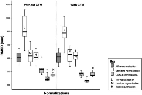
A key component of group analyses of neuroimaging data is precise and valid spatial normalization (i.e., inter-subject image registration). When patients have structural brain lesions, such as a stroke, this process can be confounded by the lack of correspondence between the subject and standardized template images. Current procedures for dealing with this problem include regularizing the estimate of warping parameters used to match lesioned brains to the template, or "cost function masking"; both these solutions have significant drawbacks. We report three experiments that identify the best spatial normalization for structurally damaged brains and establish whether differences among normalizations have a significant effect on inferences about functional activations. Our novel protocols evaluate the effects of different normalization solutions and can be applied easily to any neuroimaging study. This has important implications for users of both structural and functional imaging techniques in the study of patients with structural brain damage.

Fig. 1

An example of a ‘real’ and a simulated lesioned brain derived from this ‘real’ image used in the anatomical validation: Experiment 2. Image slices shown from top are coronal, sagittal and axial. L = left.

Fig. 2

Simulated lesions. Brain images used in the anatomical validation: Experiment 2. Starting from the top left and going clockwise the abnormalities are: 1) left anterior communicating artery stroke, 2) left anterior frontal lesion, 3) left temporo-parietal lesion, 4) multiple areas of cortical damage, 5) left occipitotemporal lesion, 6) left fronto-parietal lesion, 7) left temporo-parietal lesion, 8) left temporal lobe atrophy, 9) left occipitotemporal lesion, 10) left putamen/insula lesion.

Fig. 3

Experiment 1: anatomical landmarks. Location of anatomical landmarks shown on an exemplar brain: cortical landmarks are shown in white (n = 16, 8 each hemisphere): 2 frontal = F1, F2; 2 temporal = T1, T2; insula = In; parietal = Pa; occipital = Oc; cerebellum = Ce. Subcortical landmarks are in yellow (n = 8, 2 midpoint, 3 bilateral): Anterior commissure = AC; frontal horn = FH; occipital horn = OH; 4th ventricle = 4V; putamen = Pu.

Fig. 4

Experiment 1: comparing different normalization algorithms. Plot of the root mean square (RMS) values in millimeters comparing the normalizations of the group of ten normal images for all the cortical (n = 16) and subcortical (n = 6) landmarks. From the left of the image the first (dark gray) box-plot shows RMS values for the affine-only solution (mean—5.71, s.d—1.76), then next the three (white) standard solutions with low (L) (mean—6.14, s.d—3.2), medium (M) (mean—5.74, s.d—2.48), and high (H) (mean—5.67, s.d—1.88) regularizations. The subsequent 3 box-plots in light gray show RMS values for unified solutions with low (mean—4.50, s.d—2.17), medium (mean—4.49, s.d—2.1) and high (mean—4.67, s.d—2.04) regularizations. The black line in each box-plot indicates the group mean for each normalization solution. The open circle indicates a group outlier.

Fig. 5

Experiment 2: Normalization of lesioned brains with and without CFM. Plot of the root mean squared difference (RMSD) values in millimeters for the 14 normalizations of the group of ten simulated lesion–normal brain pairs. From the left of the image the first (dark gray) box-plot shows RMS values for the affine-only solution (mean—4.1, s.d—0.86), then next the three (white) standard solutions with low (L) (mean—8.36, s.d—1.82), medium (M) (mean—4.4, s.d—1.12) and high (H) (mean—4.31, s.d—0.77) regularizations. The subsequent 3 box-plots in light gray show RMS values for unified solutions with low (L) (mean—2.33, s.d—0.71), medium (M) (mean—1.09, s.d—0.58) and high (H) (mean—1.52, s.d—0.25) regularizations. The 7 subsequent box-plots, after the dotted line with shaded background, show the same normalization solutions with cost function masking (CFM): affine (mean—4.13, s.d—0.88), standard solutions with low (L) (mean—7.82, s.d—1.54), medium (M) (mean—4.35, s.d—1.07) and high (H) (mean—4.35, s.d—0.77) regularizations, unified solutions with low (L) (mean—1.62, s.d—0.32), medium (M) (mean—0.72, s.d—0.31) and high (H) (mean—1.57, s.d—0.34) regularizations. The black line in each box-plot indicates the group mean for each normalization solution. The open circle indicates a group outlier.

Fig. 6

The 14 normalization solutions for an individual brain, simulated brain lesion number ten from Fig. 2. The images show the brain after affine-only normalizations, standard nonlinear normalizations and unified models, with and without cost function masking. (A) The un-normalized T1 MR image of simulated lesion 10. (B) The unified models with low, medium and high regularizations. (C) The same unified models as in B above with CFM. (D) The affine-only (1) and standard normalizations with low, medium and high regularizations. (E) The same normalizations as in row D above with CFM.

Fig. 7

Experiment 3: fMRI results. Regional activation for unified > standard normalization solutions. For the group of 18 stroke patients, results are shown in color rendered onto the SPM5 single-subject brain template. In the left (L) hemisphere there was one peak in the middle superior temporal gyrus (coordinate x = − 58 y = − 14 z = 6; z score = 3.98). In the right (R) hemisphere there were 3 main peaks in the posterior, (x = 50 y = − 28 z = 0; z score = 3.63), middle (x = 58 y = − 2 z = − 12; z score = 3.72) and anterior (x = 44 y = 8 z = − 16; z score = 3.84) superior temporal sulcus.

References

1. Ardekani B., Bachman A., Strother S.C., Fujibayashi Y., Yonekura Y. Impact of inter-subjects image registration on group analysis of fMRI data. Int. Congr. Ser. 2004;1265:49–59. Ref Type: Journal (Full)
1. Ashburner J., Friston K. Multimodal image coregistration and partitioning—A unified framework. NeuroImage. 1997;6:209–217. - PubMed
1. Ashburner J., Friston K.J. Nonlinear spatial normalization using basis functions. Hum. Brain Mapp. 1999;7:254–266. - PMC - PubMed
1. Ashburner J., Friston K.J. Unified segmentation. NeuroImage. 2005;26:839–851. - PubMed
1. Ashburner J., Neelin P., Collins D.L., Evans A., Friston K. Incorporating prior knowledge into image registration. NeuroImage. 1997;6:344–352. - PubMed
Publication types