A biophysical perspective on dispersal and the geography of evolution in marine and terrestrial systems

Abstract

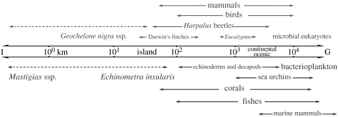
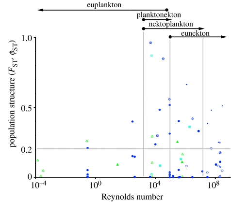
The fluid mechanics of marine and terrestrial systems are surprisingly similar at many spatial and temporal scales. Not surprisingly, the dispersal of organisms that float, swim or fly is influenced by the fluid environments of air and seawater. Nonetheless, it has been argued repeatedly that the geography of evolution differs fundamentally between marine and terrestrial taxa. Might this view emanate from qualitative contrasts between the pelagic ocean and terrestrial land conflated by anthropocentric perception of within- and between-realm variation? We draw on recent advances in biogeography to identify two pairs of biophysically similar marine and terrestrial settings--(i) aerial and marine microplankton and (ii) true islands and brackish seawater lakes--which have similar geographies of evolution. Commonalities at these scales, the largest and smallest biogeographic scales, delimit the geographical extents that can possibly characterize evolution in the remaining majority of species. The geographies of evolution therefore differ statistically, not fundamentally, between marine and terrestrial systems. Comparing the geography of evolution in diverse non-microplanktonic and non-island species from a biophysical perspective is an essential next step for quantifying precisely how marine and terrestrial systems differ and is an important yet under-explored avenue of macroecology.

Figure 1

Patterns of environmental heterogeneity which have been used to illustrate basic differences in process in marine (plankton swarm) versus terrestrial (climax forest) systems are actually two ends of a continuum, each with analogues in the other realm. (a) Simulations using cellular automata produce different distributions of groups of organisms (black)—in patches, labyrinths or interspersed with gaps—on a background of bare habitat (white; redrawn from Rietkerk et al. (2004)). The distribution of organisms depends on interactions between biotic fine-scale positive feedback (increasing in strength from left to right) and a background of coarse-scale negative feedback (constant grain and strength, therefore relatively stronger towards the left). Decreasing or increasing the grain of interactions results in smaller or larger features, respectively. Interactions between biotic (e.g. compensatory biological mechanisms, functional interactions among species), plus abiotic (e.g. disturbance, physical heterogeneity), factors are the major influences on patchiness (Krohne 2001, p. 289) and, therefore, with the scale of dispersal and gene flow, determine the shapes of geographical mosaics (sensu Thompson 2005). (b) A 1.0 km long swath from barrier reef, on the right, to patch reefs, on the left, forming a mosaic with the lighter sandy sediment bottom (17° 00′19.38″ S, 146° 16′24.16″ E); image captured from the Google Earth mapping service, copyright 2007 DigitalGlobe. (c) A 0.4 km long swath of vernal pool grassland, Merced, California (37° 23′24.02″ N, 120° 16′26.67″ W), in which the landscape changes from predominantly grassland on the left to predominantly vernal pool on the right; image captured from the Google Earth™ mapping service, © 2007 Europa Technologies.

Figure 2

Comparisons of seawater, freshwater and air as experienced by some marine (dark blue circles), aquatic (light blue squares) and terrestrial organisms (filled green triangles). (a) Variation of fluid environment, described by Reynolds number Re, with the characteristic length l and typical speeds of movement of organisms (adapted from www.natureinterface.com/e/ni05/P048/; see also Okubo 1987; Mann & Lazier 2006). Regressions of Re on l for aquatic (Re=1.79l+6.13; n=7, r=0.99, p<0.001), marine (Re=1.78l+6.11; n=26, r=0.98, p<0.001) and terrestrial (Re=1.79l+6.30; n=16, r=0.98, p<0.001) taxa were not statistically different in slope (F_2,43=0.009, p=0.99) nor intercept (F_2,45=0.500, p=0.61). (b) Four classes of movement are used by diverse marine, aquatic and terrestrial organisms due to common constraints of fluid dynamics (adapted from fig. 1 in Aleyev (1977)). A Boeing 737 (open green triangle) is included in the analyses to illustrate that movement through the air at this extreme does not deviate from the relationship in (a) or classification in (b), although attaining such values is energetically unfeasible for terrestrial organisms. The fluid environment of Typhoon class submarines is indicated by an open blue circle. The characteristic length of organisms such as jellyfish that deform their whole body to swim may vary several fold (as will any ratio thereof) depending on the stage of the swimming stroke.

Figure 3

Noise (random variation) in environmental variables is generally well described by an inverse power law, 1/f^β (where f is the frequency of variation and superscript β, a constant), the form of which varies with temporal scale and environment. (a) Schematic of predominant patterns in environmental noise predicted on the basis of empirical observations and modelling of temperature variation (redrawn from Steele (1985) and Pelletier (1997)); c, a constant. (b) Example power-spectral density of local atmospheric temperature using combined low-frequency data inferred from the Vostok ice core and high frequency data from continental instrumental records (redrawn from Pelletier (2002)). (c) White noise in precipitation may be ‘reddened’ by processes that modify water movement into and through river beds.

Figure 4

Evolutionarily averaged dispersal distances can be similar in ecologically comparable (a) terrestrial and (b) marine organisms. Dispersal scales of benthic marine primary producers (macroalgae and angiosperms; lower, light grey) and marine herbivores (invertebrates and fishes; lower, dark grey) with their terrestrial counterparts, land plants (upper, light grey) and herbivorous insects (upper, dark grey) estimated from genetic data (n=16 to 19). Redrawn from Kinlan & Gaines (2003).

Figure 5

Insular to global species ranges in terrestrial and marine taxa. Simplified schematic showing considerable overlap in the geographical ranges, from insular (I) to global (G; approximate maximum linear extent) of some terrestrial (upper, light grey) and marine (lower, dark grey) taxa, including examples of some of the most narrowly and widely distributed taxa. Harpalus (Noonan 1990), Eucalyptus (Edwards & Westoby 1996), mammals and birds (Brown et al. 1996; von Hippel 2001), Geochelone nigra ssp. (Galapagos tortoise; see http://library.sandiegozoo.org/FactSheets/tortoise_galapagos/tortoise_map.htm), echinoderms and decapods (O'Hara & Poore 2000), sea urchins (Emlet 1995), corals (Veron 2000), some whales (e.g. blue, humpback; see: http://www.jncc.gov.uk/Publications/cetaceanatlas/) and fishes (e.g. from 1°-endemic species to albacore, bigeye and yellowfin tunas; see: http://kosfic.yosu.ac.kr/kos_home/ocean_gis/FAO/mapbrief.html). Dashed lines represent, by inference, population ranges, although some populations will have larger distributions. Island, continental and oceanic scales are indicated approximately. The figure is intended to be demonstrative rather than comprehensive.

Figure 6

Relationship between Reynolds number (Re) and population subdivision (F_ST or ϕ_ST) for some marine (dark blue circles), freshwater (light blue squares) and terrestrial (green triangles) organisms. Organisms with very small Re, such as marine and aerial microplankton, are unable to influence fluid dispersal and are expected to have high gene flow (low F_ST and ϕ_ST) and very large geographical ranges. Organisms with very large Re, such as marine mammals and large birds, have locomotory abilities that far exceed the influence of fluid dispersal and are also expected to have high gene flow and very large geographical ranges. These taxa with potentially high dispersal typically have F_ST or ϕ_ST less than 0.2 (see light grey horizontal line), indicating at least one successful migrant per generation, i.e. sufficient in theory to prevent geographical differentiation. Organisms with intermediate Re, such as large insects, small birds and many reef fishes, are often able to avoid passive fluid dispersal but unable to move very large distances due to biomechanical or energetic restrictions; they are expected to have various degrees of connectivity and range-sizes, including many instances of low gene flow (high F_ST and ϕ_ST). The light grey vertical lines delimit the different classes of motility identified by Aleyev (1977). Differences in population subdivision between organisms with similar Re may indicate the influences of behaviour, life history, physical discontinuities (environmental filters), chance and other events on gene flow. Solid symbols, mitochondrial DNA; open symbols, nuclear DNA. Note that estimates of gene flow in marine mammals based on analyses of mitochondrial DNA (small solid circles) are inflated relative to those based on nuclear DNA due to female social structure (e.g. Bérubé et al. 1998; Burg et al. 1999; Durand et al. 2005). Pairs of crossed squares and circles with the same or similar Re highlight examples in which physical isolation or environmental filters contribute to high population subdivision (Bérubé et al. 1998; Dawson et al. 2002; Dawson & Hamner 2005). Crossed diamonds show examples in which life histories, in these cases vivipary or brooding or adult migration, contribute to high population subdivision (Bernardi 2000; Planes et al. 2001; Bowen et al. 2005).

References

1. Addicott W.O. Late Pleistocene marine paleoecology and zoogeography in central California. US Geol. Surv. Prof. Pap. 1966;523C:C1–C21.
1. Aleyev Y.G. Jung; The Hague, The Netherlands: 1977. Nekton.
1. Anderson M.J. Effects of patch size on colonization in estuaries: revisiting the species–area relationship. Oecologia. 1998;118:87–98. doi: 10.1007/s004420050706. - DOI - PubMed
1. Angel M.V. Biodiversity of the pelagic ocean. Conserv. Biol. 1993;7:760–772. doi: 10.1046/j.1523-1739.1993.740760.x. - DOI
1. Baldwin A.J, Moss J.A, Pakulski J.D, Catala P, Joux F, Jeffrey W.H. Microbial diversity in a Pacific Ocean transect from the Arctic to Antarctic circles. Aquat. Microb. Ecol. 2005;41:91–102.
LinkOut - more resources