Simulation of networks of spiking neurons: a review of tools and strategies

Abstract

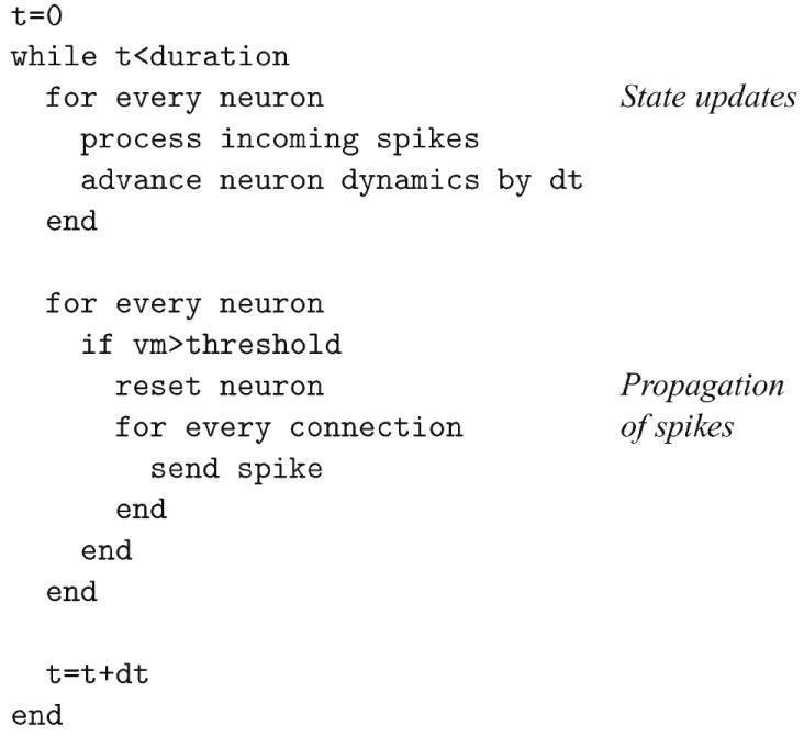
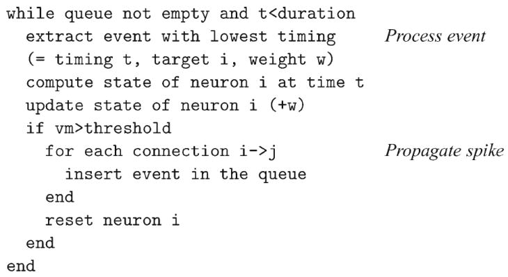
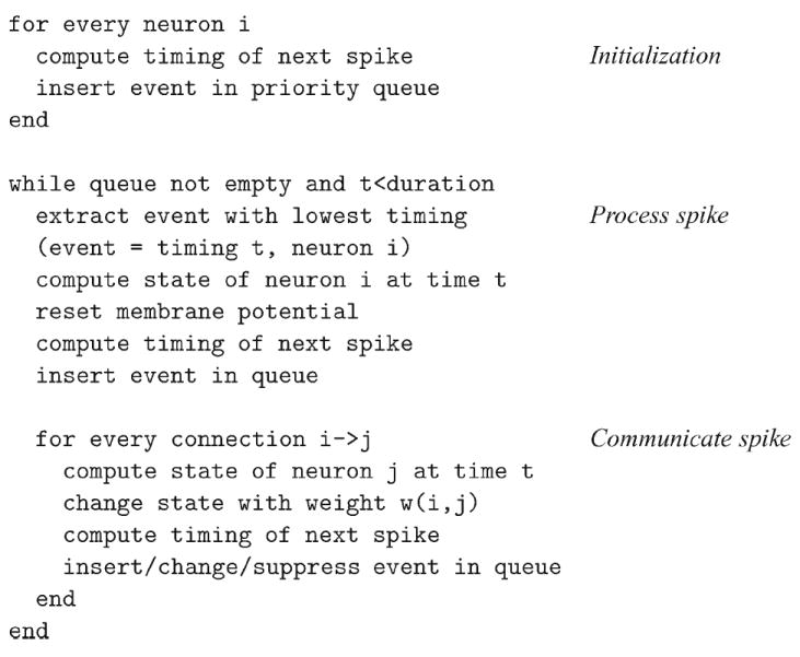
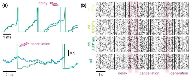
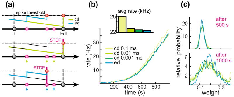
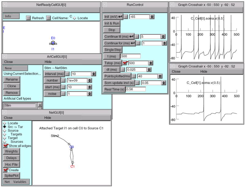
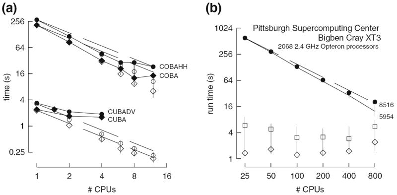
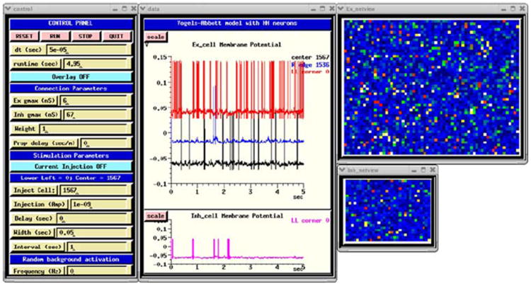
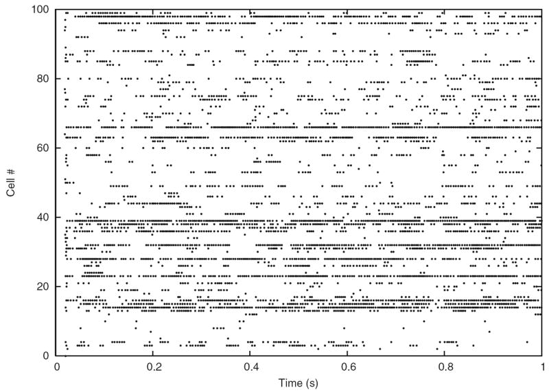
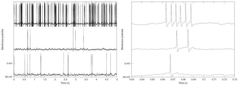
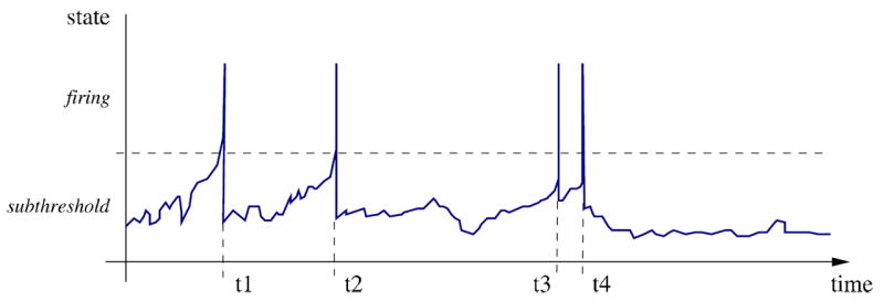
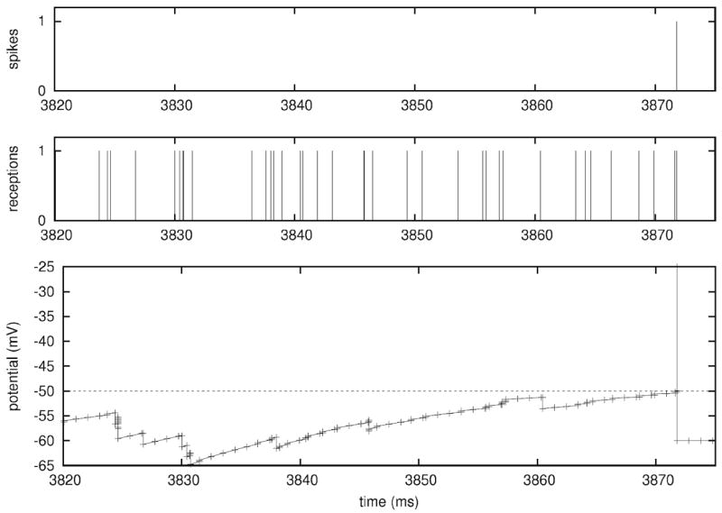
We review different aspects of the simulation of spiking neural networks. We start by reviewing the different types of simulation strategies and algorithms that are currently implemented. We next review the precision of those simulation strategies, in particular in cases where plasticity depends on the exact timing of the spikes. We overview different simulators and simulation environments presently available (restricted to those freely available, open source and documented). For each simulation tool, its advantages and pitfalls are reviewed, with an aim to allow the reader to identify which simulator is appropriate for a given task. Finally, we provide a series of benchmark simulations of different types of networks of spiking neurons, including Hodgkin-Huxley type, integrate-and-fire models, interacting with current-based or conductance-based synapses, using clock-driven or event-driven integration strategies. The same set of models are implemented on the different simulators, and the codes are made available. The ultimate goal of this review is to provide a resource to facilitate identifying the appropriate integration strategy and simulation tool to use for a given modeling problem related to spiking neural networks.

Fig. 1

A basic clock-driven algorithm

Fig. 2

A basic event-driven algorithm with instantaneous synaptic interactions

Fig. 3

A basic event-driven algorithm with non-instantaneous synaptic interactions

Fig. 4

Modelling strategies and dynamics in neuronal systems without STDP. (a) Small differences in spike times can accumulate and lead to severe delays or even cancellation (see arrows) of spikes, depending on the simulation strategy utilized or the temporal resolution within clock-driven strategies used. (b) Raster-plots of spike events in a small neuronal network of LIF neurons simulated with event-driven and clock-driven approaches with different temporal resolutions. Observed differences in neural network dynamics include delays, cancellation or generation of synchronous network events [figure modified from Rudolph and Destexhe (2007)]

Fig. 5

Dynamics in neuronal systems with STDP. (a) Impact of the simulation strategy (clock-driven: cd; event-driven: ed) on the facilitation and depression of synapses. (b) Time course and average rate (inset) in a LIF model with multiple synaptic input channels for different simulation strategies and temporal resolution. (c) Synaptic weight distribution after 500 and 1,000 s [figure modified from Rudolph and Destexhe (2007)]

Fig. 6

NEURON graphical user interface. In developing large scale networks, it is helpful to start by debugging small prototype nets. NEURON’s GUI, especially its Network Builder (shown here), can simplify this task. Also, at the click of a button the Network Builder generates hoc code that can be reused as the building blocks for large scale nets [see Chapter 11, “Modeling networks” in Carnevale and Hines (2006)]

Fig. 7

Parallel simulations using NEURON. (a) Four benchmark network models were simulated on 1, 2, 4, 6, 8, and 12 CPUs of a Beowulf cluster (6 nodes, dual CPU, 64-bit 3.2 GHz Intel Xeon with 1024 KB cache). Dashed lines indicate “ideal speedup” (run time inversely proportional to number of CPUs). Solid symbols are run time, open symbols are average computation time per CPU, and vertical bars indicate variation of computation time. The CUBA and CUBADV models execute so quickly that little is gained by parallelizing them. The CUBA model is faster than the more efficient CUBADV because the latter generates twice as many spikes (spike counts are COBAHH 92,219, COBA 62,349, CUBADV 39,280, CUBA 15,371). (b) The Pittsburgh Supercomputing Center’s Cray XT3 (2.4 GHz Opteron processors) was used to simulate a NEURON implementation of the thalamocortical network model of Traub et al. (2005). This model has 3,560 cells in 14 types, 3,500 gap junctions, 5,596,810 equations, and 1,122,520 connections and synapses, and 100 ms of model time it generates 73,465 spikes and 19,844,187 delivered spikes. The dashed line indicates “ideal speedup” and solid circles are the actual run times. The solid black line is the average computation time, and the intersecting vertical lines mark the range of computation times for each CPU. Neither the number of cell classes nor the number of cells in each class were multiples of the number of processors, so load balance was not perfect. When 800 CPUs were used, the number of equations per CPU ranged from 5954 to 8516. Open diamonds are average spike exchange times. Open squares mark average voltage exchange times for the gap junctions, which must be done at every time step; these lie on vertical bars that indicate the range of voltage exchange times. This range is large primarily because of synchronization time due to computation time variation across CPUs. The minimum value is the actual exchange time

Fig. 8

The GUI for the GENESIS implementation of the HH benchmark, using the dual-exponential form of synaptic conductance

Fig. 9

Membrane potentials for four selected neurons of the Instantaneous Conductance VA HH Model in GENESIS. (a) The entire 5 s of the simulation. (b) Detail of the interval 3.2–3.4 s

Fig. 10

Performance of NEST on Benchmarks 1-4 and an additional benchmark (5) with STDP. (a) Simulation time for one biological second of Benchmarks 1-3 distributed over two processors, spiking supressed, with a synaptic delay of 0.1 ms. The horizontal lines indicate the simulation times for the benchmarks with the synaptic delay increased to 1.5 ms. (b) Simulation time for one biological second of Benchmark 4 as a function of the minimum synaptic delay in double logarithmic representation. The gray line indicates a linear fit to the data (slope–0.8). (c) Simulation time for one biological second of Benchmark 5, a network of 11250 neurons and connection probability of 0.1 (total number of synapses: 12.7 × 10⁶) as a function of the number of processors in double logarithmic representation. All synapses static, triangles; excitatory-excitatory synapses implementing multiplicative STDP with an all-to-all spike pairing scheme, circles. The gray line indicates a linear speed-up

Fig. 11

NCS file specifications and example of simulation. (a) Hierarchy of the NCS Command File Objects. The file is ASCII-based with simple object delimiters. Brainlab scripting tools are available for repetitive structures (Drewes 2005). (b) 1-s spike rastergram of 100 arbitrarily selected neurons in the benchmark simulation

Fig. 12

Results of CSIM simulations of the Benchmarks 1 to 3 (top to bottom). The left panels show the voltage traces (in mV) of a selected neuron. For Benchmark 1 (COBA) and Benchmark 2 (CUBA) models (top two rows), the spikes superimposed as vertical lines. The right panels show the spike raster for randomly selected neurons for each of the three benchmarks

Fig. 13

Performance of PCSIM. The time needed to simulate the Benchmark 2 (CUBA) network (1 ms synaptic delay, 0.1 ms time step) for 1 s of biological time (solid line) as well as the expected times (dashed line) are plotted against the number of machines (Intel Xeon, 3.4 Ghz, 2 Mb cache). The CUBA model was simulated for three different sizes: 4000 neurons and 3.2 × 10⁵ synapses (stars), 10000 neurons and 2 × 10⁶ synapses (circles), and 20000 neurons and 20 × 10⁶ synapses (diamonds)

Fig. 14

XPPAUT interface for a network of 200 excitatory and 50 inhibitory HH neurons with random connectivity, COBA dynamical synapses. Each neuron is also given a random drive. Main window, a three-dimensional phase plot, and an array plot are shown

Fig. 15

Persistent state in an IF network with 400 excitatory and 100 inhibitory cell. XPPAUT simulation with exponential COBA synapses, sparse coupling and random drive. Excitatory and inhibitory synapses are shown as well as voltages traces from 3 neurons

Fig. 16

Speedup for model with 4 million cells and 2 billion synapses simulated with SPLIT on BG/L (from Djurfeldt et al. 2005)

Fig. 17

Raster plot showing spikes of 100 cells during the first second of activity (SPLIT simulation of Benchmark 3)

Fig. 18

Plots of the membrane potential for 3 of the 4000 cells. The right plot shows a subset of the data in the left plot, with higher time resolution (SPLIT simulation of Benchmark 3)

Fig. 19

Neuronal dynamics from a discrete-event dynamical systems perspective. Events (t1-t4), corresponding to the state variable switching from the sub-threshold to the firing dynamics, can occur at any arbitrary point in time. They correspond here to change of the neuron output that can be passed to the rest of the systems (e.g. other neurons). Internal changes (e.g. end of the refractory period) can also be described in a similar way

Fig. 20

Membrane potential of a single neuron, from a Mvaspike implementation of Benchmark 4. Top: membrane potential dynamics (impulses have been superimposed at firing time to make them more apparent). Bottom: Mvaspike simulation result typically consists of lists of events (here, spiking and reception time, top and middle panels) and the corresponding state variables at these instants (not shown). In order to obtain the full voltage dynamics, a post-processing stage is used to add new intermediary values between events (bottom trace)

Fig. 21

Example of Hodgkin-Huxley K⁺ conductance specified in ChannelML, a component of NeuroML

Fig. 22

From NeuroML to simulator

Fig. 23

Example of the use of the PyNN API to specify a network that can then be run on multiple simulators

Fig. 24

Same network model run on two different simulators using the same source code. The model considered was the Vogels-Abbott integrate-and-fire network with CUBA synapses and displaying self-sustained irregular activity states (Benchmark 2 in Appendix B). This network implemented with the PyNN simulator-independent network modelling API, and simulated using NEST (left column) and NEURON (right column) as the simulation engines. The same sequence of random numbers was used for each simulator, so the connectivity patterns were rigorously identical. The membrane potential trajectories of individual neurons simulated in different simulators rapidly diverge, as small numerical differences are rapidly amplified by the large degree of recurrency of the circuit, but the interspike interval (ISI) statistics of the populations are almost identical for the two simulators. (Top row) Voltage traces for two cells chosen at random from the population. (Second row) Spike raster plots for the first 320 neurons in the population. (Third row) Histograms of ISIs for the excitatory and inhibitory cell populations. (Bottom row) Histograms of the coefficient of variation (CV) of the ISIs

References

1. Abbott LF, Nelson SB. Synaptic plasticity: taming the beast. Nature Neuroscience. 2000;3(Suppl):1178–1283. - PubMed
1. Arnold L. Stochastic differential equations: Theory and applications. New York: J Wiley and Sons; 1974.
1. Azouz R. Dynamic spatiotemporal synaptic integration in cortical neurons: neuronal gain, revisited. Journal of Neurophysiology. 2005;94:2785–2796. - PubMed
1. Badoual M, Rudolph M, Piwkowska Z, Destexhe A, Bal T. High discharge variability in neurons driven by current noise. Neurocomputing. 2005;65:493–498.
1. Bailey J, Hammerstrom D. International Conference on Neural Networks (ICNN 88, IEEE) San Diego: 1988. Why VLSI implementations of associative VLCNs require connection multiplexing; pp. 173–180.
Publication types
LinkOut - more resources