A model of the go/no-go task

Abstract

In this article, the first explicit, theory-based comparison of 2-choice and go/no-go variants of 3 experimental tasks is presented. Prior research has questioned whether the underlying core-information processing is different for the 2 variants of a task or whether they differ mostly in response demands. The authors examined 4 different diffusion models for the go/no-go variant of each task along with a standard diffusion model for the 2-choice variant (R. Ratcliff, 1978). The 2-choice and the go/no-go models were fit to data from 4 lexical decision experiments, 1 numerosity discrimination experiment, and 1 recognition memory experiment, each with 2-choice and go/no-go variants. The models that assumed an implicit decision criterion for no-go responses produced better fits than models that did not. The best model was one in which only response criteria and the nondecisional components of processing changed between the 2 variants, supporting the view that the core information on which decisions are based is not different between them.

Figure 1

Panel A shows a representation of the sequence of events in a trial of a dual-choice task in which the stimulus is presented until a response is made. Panel B represents the nondecisional components of the response time (RT), which have a mean expressed by the T_er parameter and a range expressed by the s_t parameter. Panel C illustrates the diffusion model. The parameters represented in Panel C are a = boundary separation; z = starting point; s_z = variability in starting point across trials; v = drift rate; η = variability in the drift rate across trials; and variability in drift rate within a trial. Panels D to G (Imp = implicit boundary) show representations of the models of the go/no-go task. Panel D illustrates the single boundary model of the go/no-go task with z, T_er, and the drift rates as free parameters. Panel E illustrates the decision criteria model of the go/no-go task; it assumes an implicit negative decision boundary and a, z, and T_er as free parameters. Panel F illustrates the drift criterion model of the go/no-go task; it assumes an implicit negative decision boundary and a, z, T_er, and a constant added to all drift rates as free parameters. Panel G illustrates the drift rate model of the go/no-go task; it assumes an implicit negative decision boundary and a, z, T_er, and drift rates as free parameters.

Figure 2

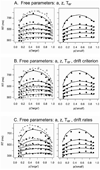
The three panels show the empirical .1, .3, .5, .7, and .9 quantiles for the response time (RT) distributions in Experiment 1. The + signs are quantile RTs plotted against accuracy values calculated for the two-choice data with the accuracy range plotted on the x-axis (−.02 to +.02). The × signs are the quantile RTs for go/no-go data. The different panels represent the fits of the different models: the decision criteria model (A); the drift criterion model (B); and the drift rate model (C). The gray blobs show variability from Monte Carlo simulations based on the model. NWe = error responses to nonwords; NWc = correct responses to nonwords; LFc = correct responses to low-frequency words; LFe = error responses to low-frequency words; MFc = correct responses to medium-frequency words; MFe = error responses to medium-frequency words; NWg = go responses to nonwords; LFg = go responses to low-frequency words; MFg = go responses to medium-frequency words.

Figure 3

The three panels show the empirical .1, .3, .5, .7, and .9 quantiles for the response time (RT) distributions in Experiment 2. The + signs are quantile RTs plotted against accuracy values calculated for the two-choice data. The × signs are the quantile RTs for go/no-go data. The different panels represent the fits of the different models: the decision criteria model (A); the drift criterion model (B); and the drift rate model (C). The gray blobs show variability from Monte Carlo simulations based on the model. NWe = error responses to nonwords; NWc = correct responses to nonwords; LFc = correct responses to low-frequency words; LFe = error responses to low-frequency words; MFc = correct responses to medium-frequency words; MFe = error responses to medium-frequency words; NWg = go responses to nonwords; LFg = go responses to low-frequency words; MFg = go responses to medium-frequency words.

Figure 4

The three panels show the empirical .1, .3, .5, .7, and .9 quantiles for the response time (RT) distributions in Experiment 3. The + signs are quantile RTs plotted against accuracy values calculated for the two-choice data. The × signs are the quantile RTs for go/no-go data. The different panels represent the fits of the different models: the decision criteria model (A); the drift criterion model (B); and the drift rate model (C). The gray blobs show variability from Monte Carlo simulations based on the model. NWe = error responses to nonwords; NWc = correct responses to nonwords; LFc = correct responses to low-frequency words; LFe = error responses to low-frequency words; MFc = correct responses to medium-frequency words; MFe = error responses to medium-frequency words; NWg = go responses to nonwords; LFg = go responses to low-frequency words; MFg = go responses to medium-frequency words.

Figure 5

The two panels show the empirical .1, .3, .5, and .9 quantiles for the RT distributions in Experiment 4. The + signs are quantile response times (RTs) plotted against accuracy values calculated for the two-choice data. The × signs are the quantile RTs for go/no-go data. The gray blobs show variability from Monte Carlo simulations based on the decision criteria model. NWe = error responses to nonwords; NWc = correct responses to nonwords; LFc = correct responses to low-frequency words; LFe = error responses to low-frequency words; MFc = correct responses to medium-frequency words; MFe = error responses to medium-frequency words; NWg = go responses to nonwords; LFg = go responses to low-frequency words; MFg = go responses to medium-frequency words.

Figure 6

Quantile-probability functions for the averaged data in Experiment 5. The panels on the left correspond to “large” responses; the filled dots represent the data from the two-choice task, and the open dots represent the data from the go/no-go procedure. The panels on the right represent “small” responses in the two-choice procedure. The empirical data are the same across the three rows, but the fits of the models change. The solid line represents the fit of the model to the two-choice data, and the dashed line represents the fit of the model to the go/no-go data. The quantile-probability functions displayed in this figure better allow us to observe the effects of the task on the latency and accuracy data simultaneously. Given the large number of conditions, we use this displaying method instead of the confidence dots shown in the previous experiments. RT = response time.

Figure 7

Quantile-probability functions for the averaged data in Experiment 6. The panels on the left correspond to “old” responses; the filled dots represent the data from the two-choice task, and the open dots represent the data from the go/no-go procedure. The panels on the right represent “new” responses in the two-choice procedure; in these right panels, the “new” responses to low-frequency two-presentation words are represented by a single point (the median), because there were not enough responses per subject to estimate the quantiles for the response time (RT) distribution. The empirical data are the same across the three rows, but the fits of the models change. The solid line represents the fit of the model to the two-choice data, and the dashed line represents the fit of the model to the go/no-go data.

References

1. Balota DA, Spieler DH. Lexicality, frequency and repetition effects: Beyond measures of central tendency. Journal of Experimental Psychology: General. 1999;128:32–55. - PubMed
1. Basso MA, Wurtz RH. Modulation of neuronal activity in superior colliculus by changes in target probability. Journal of Neuroscience. 1998;18:7519–7534. - PMC - PubMed
1. Boldini A, Russo R, Avons SE. One process is not enough! A speed-accuracy tradeoff study of recognition memory. Psychonomic Bulletin & Review. 2004;11:353–361. - PubMed
1. Busemeyer JR, Townsend JT. Decision field theory: A dynamic cognitive approach to decision making. Psychological Review. 1993;100:432–459. - PubMed
1. Cattell J. The time taken up by cerebral operations. Mind. 1886;11:277–282. 524–538.
Publication types