

The relation between color discrimination and color constancy: when is optimal adaptation task dependent?
- PMID: 17716005
- PMCID: PMC2671007
- DOI: 10.1162/neco.2007.19.10.2610
The relation between color discrimination and color constancy: when is optimal adaptation task dependent?
Abstract
Color vision supports two distinct visual functions: discrimination and constancy. Discrimination requires that the visual response to distinct objects within a scene be different. Constancy requires that the visual response to any object be the same across scenes. Across changes in scene, adaptation can improve discrimination by optimizing the use of the available response range. Similarly, adaptation can improve constancy by stabilizing the visual response to any fixed object across changes in illumination. Can common mechanisms of adaptation achieve these two goals simultaneously? We develop a theoretical framework for answering this question and present several example calculations. In the examples studied, the answer is largely yes when the change of scene consists of a change in illumination and considerably less so when the change of scene consists of a change in the statistical ensemble of surface reflectances in the environment.
Figures


 ) as a function of the gain parameter for four noise levels.
 decreases when the illuminant intensity is changed and the adaptation parameters are held constant. Here the x-axis indicates the single scene illuminant intensity used in the calculations for the corresponding point. The open circles and dashed line show how constancy performance
  decreases when the test illuminant intensity is changed and the adaptation parameters are held fixed across the change. Here the x-axis indicates the test illuminant intensity, with the reference illuminant intensity held fixed at 100. All calculations performed with adaptation parameters held fixed (g = 0.021, n = 2) and for σn = 0.05. The surface distribution had parameters μr = 0.5 and σr = 0.3.
 and for various optimizations of the steepness parameter n (see the text). Each set is for a different noise level (σn = 0.01, 0.025, 0.05, 0.075, 0.10), with the set closest to the upper right of the plot corresponding to the lowest noise level. The reference illuminant had intensity eref = 100, and the test illuminant had intensity etest = 160. The surface ensemble was specified by μr = 0.5 and σr = 0.3 and was common to both the reference and test environments. Both and were evaluated with respect to draws from this surface ensemble. The gain parameter was held fixed at g = 0.02045. The steepness parameter for the reference environment was n = 4.5. Parameters g = 0.02045 and n = 4.5 optimize discrimination performance for the reference environment when σn = 0.05. The open circles connected by the dashed line show the performance points that could be obtained for each noise level if there were no trade-off between discrimination and constancy. (Right) Equivalent trade-off noise plotted against visual noise level σn. See the discussion in the text.
 for two visual environments characterized by a common illuminant but different surface ensembles (surface ensemble 1 and surface ensemble 2). The illuminant intensity was 100. In surface ensemble 1, μr = 0.5 and σr = 0.3. In surface ensemble 2, μr = 0.7 and σr = 0.1. The histogram under the graph shows the distributions of reflected light intensities for the two ensembles. The graph shows the resultant visual response function for each case. The solid line corresponds to surface ensemble 1 and the dotted line to surface ensemble 2. The histogram to the left of the graph shows the response distribution for surface ensemble 1 under the surface ensemble 1 response function, while the histogram to the right shows the response distribution for surface ensemble 2 under the surface ensemble 2 response function. All calculations done for σn = 0.05 and e = 100. In evaluating for surface ensemble 1, performance was averaged over draws from surface ensemble 1; in evaluating for surface ensemble 2, performance was averaged over draws from surface ensemble 2. The dashed lines show how the visual response to the light intensity reflected from a fixed surface varies with the change in adaptation parameters. (Since the illuminant is held constant, a fixed surface corresponds to a fixed light intensity.)
 in the same format as the left panel of Figure 5. When the adaptation parameters are chosen to optimize discrimination () for the test environment (surface ensemble 2), constancy performance () is poor (lower right end of each set of connected dots). When the adaptation parameters are chosen to optimize constancy, discrimination performance is poor (upper left end of each set.) The connected sets of dots show how performance on the two tasks trades off for five noise levels σn = 0.01, 0.025, 0.05, 0.075, 0.10. Surface ensemble parameters and illuminant intensty are given in the caption for Figure 6. In evaluating , the adaptation parameters used for computing responses in the reference environment (surface ensemble 1) were held fixed at g = 0.02045 and n = 4.5. These parameters optimize discrimination performance for the reference environment when σn = 0.05. (Right) Equivalent trade-off noise plotted against noise level σn.
 versus trade-off curves with respect to illuminant changes. The reference environment illuminant was D65; the test environment illuminants were (from top to bottom) the blue, yellow, and red illuminants. The reference and test environment surface ensembles were the baseline surface ensemble in each case. The individual sets of connected points show performance for noise levels σn,, = 0.10, 0.15, 0.20, 0.25, 0.30, 0.35, 0.40, 0.45, 0.50. In evaluating , the adaptation parameters for the reference environment were those that optimized discrimination performance in the reference environment. These parameters were optimized separately for each noise level. (Right panels) Equivalent tradeoff noise plotted against noise level σn.
 , the adaptation parameters for the reference environment were those that optimized discrimination performance in the reference environment. These parameters were optimized separately for each noise level.
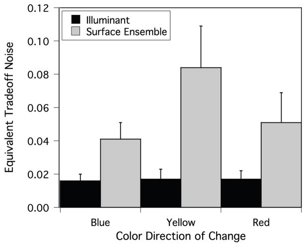
References
-
- Bindman D, Chubb C. Mechanisms of contrast induction in heterogeneous displays. Vision Research. 2004;44:1601–1613. - PubMed
-
- Brainard DH. Colorimetry. In: Bass M, editor. Handbook of optics, Vol. 1:Fundamentals, techniques, and design. New York: McGraw-Hill; 1995. pp. 1–54.
-
- Brainard DH. Color vision theory. In: Smelser NJ, Baltes PB, editors. International encyclopedia of the social and behavioral sciences. Vol. 4. Oxford: Elsevier; 2001. pp. 2256–2263.
-
- Brainard DH. Color constancy. In: Chalupa L, Werner J, editors. The visual neurosciences. Vol. 1. Cambridge, MA: MIT Press; 2004. pp. 948–961.
-
- Brainard DH, Freeman WT. Bayesian color constancy. Journal of the Optical Society of America A. 1997;14:1393–1411. - PubMed
Publication types
MeSH terms
Grants and funding
LinkOut - more resources
Full Text Sources