Simulation of Ca2+ movements within the sarcomere of fast-twitch mouse fibers stimulated by action potentials

Abstract

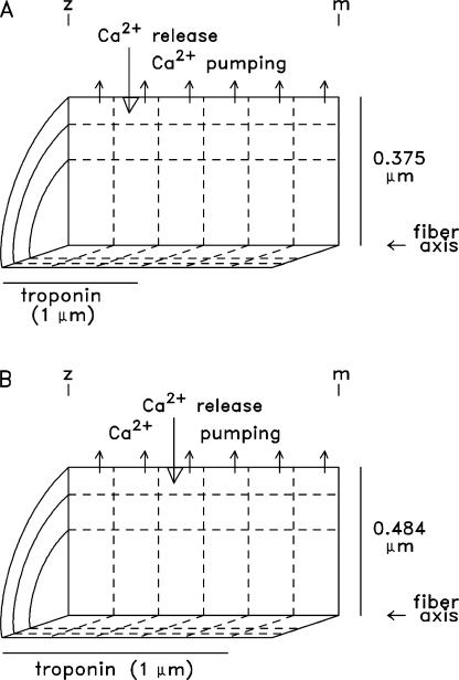
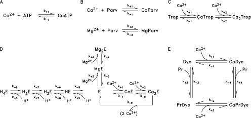
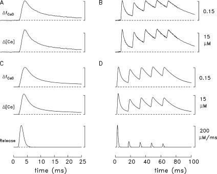
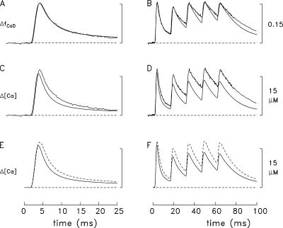
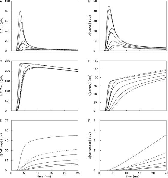
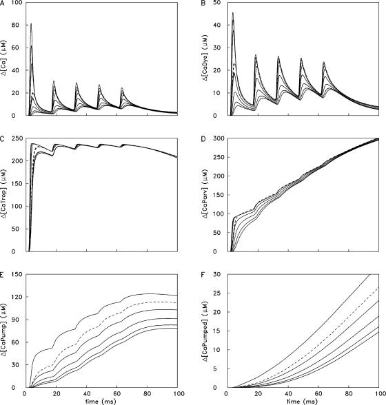
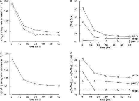
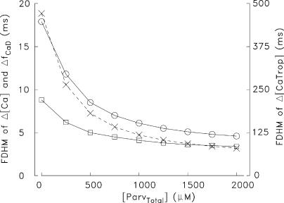
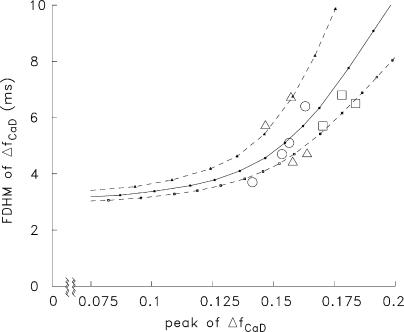
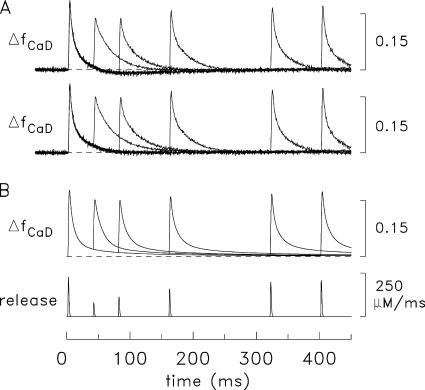
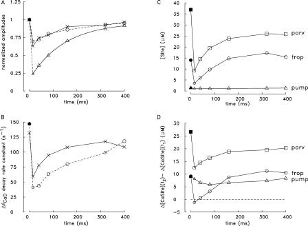
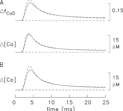
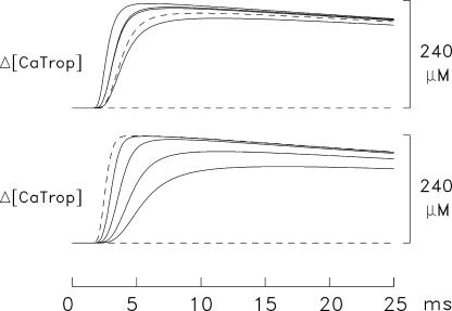
Ca(2+) release from the sarcoplasmic reticulum (SR) of skeletal muscle takes place at the triadic junctions; following release, Ca(2+) spreads within the sarcomere by diffusion. Here, we report multicompartment simulations of changes in sarcomeric Ca(2+) evoked by action potentials (APs) in fast-twitch fibers of adult mice. The simulations include Ca(2+) complexation reactions with ATP, troponin, parvalbumin, and the SR Ca(2+) pump, as well as Ca(2+) transport by the pump. Results are compared with spatially averaged Ca(2+) transients measured in mouse fibers with furaptra, a low-affinity, rapidly responding Ca(2+) indicator. The furaptra Deltaf(CaD) signal (change in the fraction of the indicator in the Ca(2+)-bound form) evoked by one AP is well simulated under the assumption that SR Ca(2+) release has a peak of 200-225 microM/ms and a FDHM of approximately 1.6 ms (16 degrees C). Deltaf(CaD) elicited by a five-shock, 67-Hz train of APs is well simulated under the assumption that in response to APs 2-5, Ca(2+) release decreases progressively from 0.25 to 0.15 times that elicited by the first AP, a reduction likely due to Ca(2+) inactivation of Ca(2+) release. Recovery from inactivation was studied with a two-AP protocol; the amplitude of the second release recovered to >0.9 times that of the first with a rate constant of 7 s(-1). An obvious feature of Deltaf(CaD) during a five-shock train is a progressive decline in the rate of decay from the individual peaks of Deltaf(CaD). According to the simulations, this decline is due to a reduction in available Ca(2+) binding sites on troponin and parvalbumin. The effects of sarcomere length, the location of the triadic junctions, resting [Ca(2+)], the parvalbumin concentration, and possible uptake of Ca(2+) by mitochondria were also investigated. Overall, the simulations indicate that this reaction-diffusion model, which was originally developed for Ca(2+) sparks in frog fibers, works well when adapted to mouse fast-twitch fibers stimulated by APs.

Figure 1.

Cut-away view of a half sarcomere of one myofibril showing the arrangement of the 18 equal-volume compartments (six longitudinal × three radial) in the simulations at a sarcomere length of 4 μm (A) and 2.4 μm (B). SR Ca²⁺ release enters the myoplasm near the middle of the thin filament in the outer compartment row (large downward arrow); Ca²⁺ pump activity occurs within all compartments in the outer row (small upward arrows). In both arrangements, troponin is restricted to the compartments located within 1 μm of the z-line (the region containing thin filaments, average length ∼1 μm). Because the buffer concentrations in Table I are averages over the entire myoplasmic volume, the actual compartment concentration of troponin is 2.0 (A) or 1.2 (B) times the value listed in Table I, and the actual compartment concentration of Ca²⁺ pump molecules is three times (both A and B) the value listed in Table I. In both parts, the vertical and horizontal calibrations are different and not to scale.

Figure 2.

Reaction schemes for ATP (A), parvalbumin (B), troponin (C), the SR Ca²⁺ pump (D), and furaptra (=Dye; E). Table I gives the total reactant concentrations and Table II the reaction rate constants. With the resting values of free [Ca²⁺], free [Mg²⁺], and pH in Table I, the fractional amounts of the various reactants at rest are (A) ATP (1.000), CaATP (0.000); (B) Parv (0.062), CaParv (0.258), MgParv (0.680); (C) Trop (0.993), CaTrop (0.006), Ca₂Trop (0.001); (D) E (0.006), CaE (0.006), Ca₂E (0.004), MgE (0.123), Mg₂E (0.123), HE (0.062), H₂E (0.615), H₃E (0.062), H₄E (0.001); (E) Dye (0.451), CaDye (0.000), PrDye (0.548), CaPrDye (0.000). The resting fraction of furaptra in the protein-bound form, 0.548, is approximately consistent with that estimated from furaptra's apparent myoplasmic diffusion coefficient, 0.68 × 10⁻⁶ cm²s⁻¹, measured in frog twitch fibers at 16°C (Konishi et al., 1991). From this diffusion coefficient, Zhao et al. (1996) estimated that the fraction of furaptra in the protein-bound form in resting frog fibers is 0.58.

Figure 3.

Spatially averaged responses elicited by a single AP (left) and a 67-Hz train of 5 APs (right) initiated at 0 time. (A and B) Experimental Δf_CaD and Δ[Ca²⁺] responses averaged from four fibers in which Δf_CaD was relatively free of movement artifacts; Δ[Ca²⁺] was calculated from Δf_CaD with Eq. 3 in Materials and Methods. The mean sarcomere length was 3.8 μm (range, 3.7–3.9 μm) and the mean myoplasmic concentration of furaptra was 89 μM (range, 64–113 μM). Fiber identification numbers: 032596.2, 040596.1, 040896.1, and 040996.3. (C and D) Δf_CaD and Δ[Ca²⁺] responses averaged over the 18 compartments in the multicompartment simulations. The bottom traces show the release fluxes used to drive the simulations. The peaks of the release fluxes are 205 μM/ms in C and 208, 53, 45, 38, and 32 μM/ms in D (APs 1–5, respectively); the FDHM of all release fluxes is 1.6 ms. The values of Δ[Ca_Total] are 349 μM in C and 354, 90, 76, 66, and 55 μM in D.

Figure 4.

Comparison of spatially averaged waveforms in the experiments and simulations. (A) superposition of the Δf_CaD waveforms in Fig. 3 C and Fig. 3 A (noise-free and slightly noisy traces, respectively). (C) Superposition of the Δ[Ca²⁺] waveform in Fig. 3 C (noise-free trace) and the Δ[Ca²⁺] waveform in Fig. 3 A (noisy trace). (E) Superposition of the Δ[Ca²⁺] waveform in Fig. 3 C (continuous trace) and Δ[Ca²⁺] calculated with Eq. 3 from the Δf_CaD waveform in Fig. 3 C (dashed trace). (B, D, and F) Similar presentation for the measurements and simulations in Fig. 3 (B and D).

Figure 5.

Ca²⁺ concentration changes in the 18 compartments in the simulation of Fig. 3 C. Δ[CaDye] includes both protein-free and protein-bound furaptra (Fig. 2 E); Δ[CaTrop] and Δ[CaPump] include the Ca²⁺ ions that are both singly and doubly bound to these buffers (Fig. 2, C and D). In each panel, peak amplitudes decline with distance from the release compartment; dashed traces denote changes in compartments adjacent to the z-line. In several panels, there is an apparent grouping of the traces in triplets, which corresponds to the three radial compartments at a given longitudinal location; at some longitudinal locations, the changes in the three radial compartments are indistinguishable. To facilitate comparisons among panels, the calibrations of the ordinates are referred to the total concentrations listed in Table I, which are spatially averaged. Because troponin and the Ca²⁺ pump are not located in all compartments, the simulated amplitudes of Δ[CaTrop] and Δ[CaPump] in their respective compartments are larger than shown in the plots by the ratio of the total site concentrations in these compartments to the spatially averaged concentrations (see Fig. 1, legend).

Figure 6.

Ca²⁺ concentration changes in the 18 compartments in the simulation of Fig. 3 D. The presentation is like that in Fig. 5.

Figure 7.

Analysis of changes in spatially averaged waveforms during a five-shock, 67-Hz stimulus (A, measurements; A–D, simulations). (A) The Δf_CaD waveforms in Fig. 3 (B and D) were analyzed to estimate the rate constants characterizing the early decay of the changes evoked by the five APs. For each change, a decaying single-exponential function without an offset was fitted to the falling phase of Δf_CaD during a 4–5-ms period that began 1–1.5 ms after peak; the time points that specify the beginning and end of each fitting period are denoted t₁ and t₂. The fitted rate constants are plotted vs. the times of the corresponding external shocks (open circles, measurements; X's, simulations). (B) Repeat of the analysis in A for the Δ[Ca²⁺] waveform in Fig. 3 D; for each evoked change, rate constants were again determined between t₁ and t₂. (C) [Site] denotes the simulated spatially averaged concentration of sites on troponin (circles), parvalbumin (squares), and the Ca²⁺ pump (triangles) that are not bound with Ca²⁺, Mg²⁺, or H⁺ at time t₁; the values were determined from the simulations for each of the five evoked changes. (D) Simulated values of Δ[CaSite](t₂) − Δ[CaSite](t₁), defined as the change in the spatially averaged concentration of Ca²⁺ bound to troponin (circles), parvalbumin (squares), and the pump (triangles) between times t₁ and t₂. As in C, the values were determined from the multicompartment simulations for each of the five evoked changes.

Figure 8.

Effect of [Parv_Total] (the total concentration of the Ca²⁺/Mg²⁺ sites on parvalbumin) on the values of FDHM of spatially averaged Δf_CaD and Δ[Ca²⁺] (circles and squares, respectively, calibrated on the lefthand ordinate) and of spatially averaged Δ[CaTrop] (X points, calibrated on the righthand ordinate) in the multicompartment simulations. At each value of [Parv_Total], the value of R in Eq. 1 was adjusted to give peak Δf_CaD = 0.155, the value in column 2 of Table IV, A; no changes were made to other simulation variables.

Figure 9.

Relation between the peak amplitude and FDHM of spatially averaged Δf_CaD in the measurements and simulations. The large symbols show results from 11 rested EDL fibers stimulated by a single AP; circles, squares, and triangles give the values from the four fibers of Fig. 3 (A and B), the three fibers of Fig. 10 A, and the remaining fibers of this study, respectively. The curves through the small filled symbols show the relations determined in the multicompartment simulations with many values of R in Eq. 1 at three values of [Ca²⁺]_R: 150 nM (top curve), 50 nM (the standard value in the simulations; middle curve), and 0 nM (bottom curve). For the middle curve, the range in release fluxes that corresponds to the range in the experimental amplitudes of Δf_CaD is 191–233 μM/ms.

Figure 10.

Spatially averaged Δf_CaD responses with a two-AP protocol with waiting periods of 40, 80, 160, 320, and 400 ms between APs. (A) Δf_CaD responses averaged from three EDL fibers (top) and these responses after correction for a small movement artifact by the method described in the text (bottom). A rest period of 1 min was used between repetitions of the paired stimuli. Fiber identification numbers: 021097.1, 042597.1, and 042597.2. (B) Top: simulated multicompartment Δf_CaD responses to mimic the lower traces in A; bottom: the Ca²⁺ release waveforms used to drive the simulations. The release flux amplitudes are 227 μM/ms for the conditioning stimulus and 0.358, 0.498, 0.703, 0.871, and 0.917 times that of the conditioning pulse (waiting periods of 40, 80, 160, 320, and 400 ms, respectively).

Figure 11.

Analysis of measured and simulated responses with the two-AP protocol. (A) The large circles show the amplitudes of the measured Δf_CaD signals in Fig. 10 A (bottom traces) normalized by 0.178, the mean amplitude evoked by the conditioning stimulus (filled circle, t = 0 ms); each Δf_CaD amplitude was determined as the peak of Δf_CaD minus its starting value on the Δf_CaD trace evoked by the conditioning stimulus. The small circle at t = 15 ms shows the normalized amplitude averaged from the responses of the two fibers of Fig. 10 A that had measurements with a 15-ms waiting period between APs. The X's show similar information for Δf_CaD in the simulations of Fig. 10 B, as well as for a simulation with a 15-ms waiting period. The triangles show the amplitudes of the release fluxes in the simulations normalized by the release flux of the conditioning stimulus (227 μM/ms). The curve through the triangles is a least-squares fit of the points at t ≥ 40 ms with the function f(t) = R0 + (Rmax − R0) · (1 − exp(−r · t)). The fitted values of R0, Rmax, and r are 0.164, 0.965, and 6.87 s⁻¹, respectively. (B) Decay rate constants of Δf_CaD in the measurements (circles) and simulations (X's), determined as in Fig. 7 (A and B). (C and D) Values of [Site] and Δ[CaSite](t₂) − Δ[CaSite](t₁), determined as in Fig. 7 (C and D).

Figure 12.

Simulations of spatially averaged responses evoked by one AP at sarcomere lengths of 2.4 μm (dashed traces) and 4.0 μm (continuous traces). (A) The top pair of traces shows Δf_CaD and the bottom pair Δ[Ca²⁺], averaged over the 18 compartments. (B) Single-compartment estimates of Δ[Ca²⁺] obtained with Eq. 3 from the Δf_CaD traces in A. The modifications of the model for the multicompartment simulation at sarcomere length = 2.4 μm are described in the text (see also Fig. 1 B). The Ca²⁺ release flux was identical to that in Fig. 3 C.

Figure 13.

Simulated families of Δ[CaTrop] waveforms at a sarcomere length of 2.4 μm with two Ca²⁺ release locations: the middle of the thin filament (top) and adjacent to the z-line (bottom). These locations approximate the location of the triadic junctions in mammalian and amphibian fibers, respectively. Each waveform represents an average over the three radial compartments at one of the five longitudinal locations of the 15 troponin-containing compartments; these are centered at 0.1, 0.3, 0.5, 0.7, and 0.9 μm from the z-line. As in Fig. 5 C, Δ[CaTrop] includes changes in both the singly and doubly bound Ca²⁺ states of troponin, and the concentration change on the ordinate is referred to the entire myoplasmic volume. In each panel, the peak amplitudes decline with distance from the release compartment; the dashed trace shows the result closest to the z-line. The SR Ca²⁺ release function was identical to that in Fig. 3 C.

References

1. Baylor, S.M., and S. Hollingworth. 1998. Model of sarcomeric Ca2+ movements, including ATP Ca2+ binding and diffusion, during activation of frog skeletal muscle. J. Gen. Physiol. 112:297–316. - PMC - PubMed
1. Baylor, S.M., and S. Hollingworth. 2003. Sarcoplasmic reticulum calcium release compared in slow- twitch and fast-twitch fibres of mouse muscle. J. Physiol. 551:125–138. - PMC - PubMed
1. Baylor, S.M., W.K. Chandler, and M.W. Marshall. 1983. Sarcoplasmic reticulum calcium release in frog skeletal muscle fibres estimated from arsenazo III calcium transients. J. Physiol. 344:625–666. - PMC - PubMed
1. Blinks, J.R., R. Rudel, and S.R. Taylor. 1978. Calcium transients in isolated amphibian skeletal muscle fibres: detection with aequorin. J. Physiol. 277:291–323. - PMC - PubMed
1. Brown, I.E., D.H. Kim, and G.E. Loeb. 1998. The effect of sarcomere length on triad location in intact feline caudofemoralis muscle fibres. J. Muscle Res. Cell Motil. 19:473–477. - PubMed
Publication types