. 2007 Aug 29;27(35):9354-68.
doi: 10.1523/JNEUROSCI.1110-06.2007.

Evidence for the flexible sensorimotor strategies predicted by optimal feedback control

Affiliations

Evidence for the flexible sensorimotor strategies predicted by optimal feedback control

Dan Liu et al. J Neurosci. .

Abstract

Everyday movements pursue diverse and often conflicting mixtures of task goals, requiring sensorimotor strategies customized for the task at hand. Such customization is mostly ignored by traditional theories emphasizing movement geometry and servo control. In contrast, the relationship between the task and the strategy most suitable for accomplishing it lies at the core of our optimal feedback control theory of coordination. Here, we show that the predicted sensitivity to task goals affords natural explanations to a number of novel psychophysical findings. Our point of departure is the little-known fact that corrections for target perturbations introduced late in a reaching movement are incomplete. We show that this is not simply attributable to lack of time, in contradiction with alternative models and, somewhat paradoxically, in agreement with our model. Analysis of optimal feedback gains reveals that the effect is partly attributable to a previously unknown trade-off between stability and accuracy. This yields a testable prediction: if stability requirements are decreased, then accuracy should increase. We confirm the prediction experimentally in three-dimensional obstacle avoidance and interception tasks in which subjects hit a robotic target with programmable impedance. In additional agreement with the theory, we find that subjects do not rely on rigid control strategies but instead exploit every opportunity for increased performance. The modeling methodology needed to capture this extra flexibility is more general than the linear-quadratic methods we used previously. The results suggest that the remarkable flexibility of motor behavior arises from sensorimotor control laws optimized for composite cost functions.


Figures
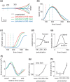
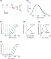
Figure 1.
Figure 1.
a, Average hand paths in experiment 1. The vertical marks show where the hand was at each perturbation time. Trajectory averaging was done as follows. The trajectory data from each individual trial were smoothed with a cubic spline (“csaps” function in the Matlab Spline Toolbox, smoothing parameter 0.001), and resampled at 100 points equally spaced in time. Analytical derivatives of the cubic spline were also computed at these 100 points, yielding velocities and accelerations. The resampled data were averaged separately in each condition. b, Tangential speed profiles for the hand paths shown in a. c, Corrective (forward) movement. The backward-perturbed trials have been mirrored around the horizontal axis and pooled with the corresponding forward-perturbed trials. The color code is the same as given in the legend in a. d, Undershoot, defined as endpoint error in the direction indicated in the plot. SEs are computed as described in Materials and Methods. e, Positional variance of the hand trajectories in unperturbed trials. Variances at each point in time are computed separately for each subject (from the resampled data), and then averaged over subjects, and the square root is plotted. f, Acceleration in the forward direction. For each perturbation time, the corresponding curve is aligned on the time when forward acceleration reached 5% of peak forward acceleration. g, Movement duration. h, Percentage of time-out errors, as signaled during the experiment. Note that for data analysis purposes, we increased the threshold on movement duration by 100 ms.
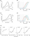
Figure 2.
Figure 2.
a–e, Same as the corresponding subplots of Figure 1, but for data generated by our optimal feedback control model. The dashed lines in c show predictions of a different optimal control model, in which movement duration is not adjusted when a perturbation arises. There is no dashed line for the 100 ms perturbation (red), because in that condition subjects did not increase the movement duration. f, Corrective movements predicted by the modified minimum-jerk model.
Figure 3.
Figure 3.
a, c, Optimal feedback gains, each scaled by its maximum value. The stop condition is shown in a; the hit condition is shown in c. b, Corrective movements predicted by the optimal feedback controller in the hit condition. d, Velocity of the corrective movements predicted in the hit condition. Note that velocity is not reduced to zero at the end of the movement, especially for the 300 ms perturbation. e, SD of the undershoot in the model and all three experiments. The SD was computed separately for each subject and perturbation time, and then averaged over subjects (by the ANOVA procedure) (see Materials and Methods). In unperturbed trials (“none”), we computed variability along the perturbation axis for the corresponding experiment, although these trials were unperturbed.
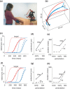
Figure 4.
Figure 4.
a, Setup for experiment 2. Subjects make a movement from the starting position receptacle to a target attached to the robot, while clearing a horizontal obstacle (bookshelf). The robot may displace the target by 9 cm left or right during the movement. b, Average hand paths in the stop condition of experiment 2. Trajectory averaging was done in a way similar to experiment 1, except that we now used a zero-phase-lag fourth-order Butterworth filter. The color code is the same as before: black, baseline; red, early perturbation; blue, late perturbation. c, Corrective movements in experiment 2. Dashed lines, Hit condition; solid lines, stop condition. d, Undershoot in experiment 2. e, Movement duration in experiment 2. f, Corrective movements in experiment 3. g, Undershoot in experiment 3. h, Movement duration in experiment 3.
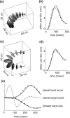
Figure 5.
Figure 5.
a, Spatial variability of unperturbed hand paths in experiment 2. The ellipsoids correspond to ±2 SDs in each direction. Aligning three-dimensional trajectories for the purpose of computing variance is nontrivial and was done as follows. We first resampled all movements for a given subject at 100 points equally spaced along the path, and found the average trajectory. Then, for each point along the average trajectory, we found the nearest sample point from each individual trajectory. These nearest points were averaged to recompute the corresponding point along the average trajectory, and the procedure was repeated until convergence (which only takes 2–3 iterations). In this way, we extracted the spatial variability of the hand paths, independent of timing fluctuations. That is why the covariance ellipsoids are flat in the movement direction. b, Variability per dimension, for the stop (solid) and hit (dashed) conditions in experiment 2. At each point along the path, this quantity was computed as the square root of the trace of the covariance matrix for the corresponding ellipsoid, divided by 3. To plot variability as a function of time, we resampled back from equal-space to equal-time intervals. c, d, Same as subplots (a, b) but for experiment 3. e, Normalized target acceleration in the lateral direction, lateral hand position, and hand position in the forward direction (positive is toward the robot). Dashed lines, Hit condition; solid lines, stop condition. Note that the onset of hand acceleration occurs before the movement reversal in the forward direction.
Figure 6.
Figure 6.
a, Endpoint SD in different directions, experiments 2 and 3, unperturbed trials. Black, Lateral direction; white, vertical direction (coordinates relative to the target); gray, vertical direction (absolute coordinates). In experiment 3, the relative and absolute endpoint positions are different in the vertical direction, because the target is falling and the variability in movement duration causes variability in vertical target position at the end of the movement. b, Lateral velocity immediately before contact with the robot, in late perturbation trials. c, Wrist contribution to the lateral correction, in a pilot experiment with 10 subjects. The main difference from experiment 2 was that the wrist was not braced. The lateral correction could be accomplished with humeral rotation (resulting mostly in translation of the hand-held pointer) or wrist flexion/extension (resulting in rotation of the pointer in the horizontal plane). The pointer was held in such a way that the Polhemus sensor was near the wrist. Therefore, the lateral displacement of the sensor on perturbed trials (relative to the average trajectory on unperturbed trials) can be used as an index of how much humeral rotation contributes to the correction. The displacement of the tip of the pointer is defined as the total correction. The difference between the two is the contribution of the wrist. Dividing the latter by the total correction, and multiplying by 100, we obtain the percentage wrist contribution.
Figure 7.
Figure 7.
a, Corrective movements of the more general optimal feedback control model. The solid and dashed lines correspond to the stop and hit conditions, respectively. The hand is restricted to a grid of discrete states; however, the dynamics are stochastic, and so the average (over 1000 simulated trials) is smooth, although the individual trajectories have a staircase pattern. b, c, Undershoot and movement duration in the stop and hit conditions for different perturbation times. Same format as the experimental data in Figure 4.
Figure 8.
Figure 8.
Hand positional variance on unperturbed trials, measured along the perturbation direction. Trajectories are aligned at equal intervals along the movement path to compute variance. The solid line (baseline) is the variance in blocks without perturbations. The dashed line (adapted) is the variance in blocks with 66% perturbations. Data from the hit and stop conditions are averaged.

References

    1. Anderson F, Pandy M. Dynamic optimization of human walking. J Biomech Eng. 2001;123:381–390. - PubMed
    1. Bernstein N. Oxford: Pergamon; 1967. The coordination and regulation of movements.
    1. Bertsekas D. Ed 2. Bellmont, MA: Athena Scientific; 2001. Dynamic programming and optimal control.
    1. Bizzi E, Hogan N, Mussa-Ivaldi F, Giszter S. Does the nervous system use equilibrium-point control to guide single and multiple joint movements? Behav Brain Sci. 1992;15:603–613. - PubMed
    1. Burdet E, Osu R, Franklin D, Milner T, Kawato M. The central nervous system stabilizes unstable dynamics by learning optimal impedance. Nature. 2001;414:446–449. - PubMed

Publication types

LinkOut - more resources