A biologically realistic model of contrast invariant orientation tuning by thalamocortical synaptic depression

Abstract

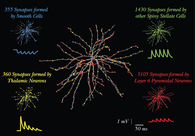
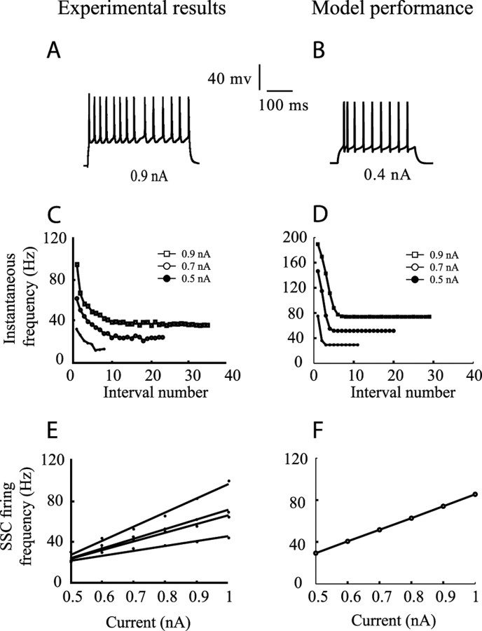
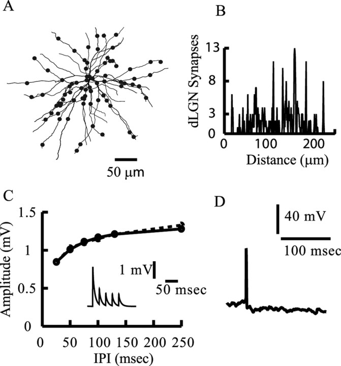
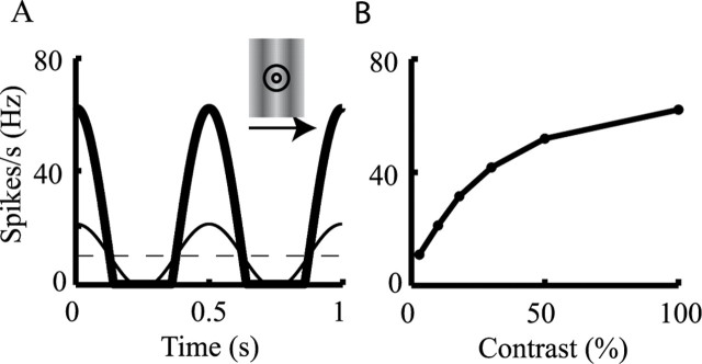
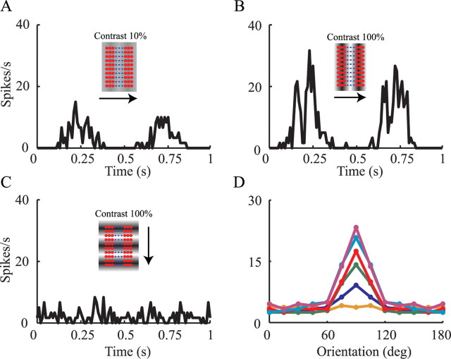
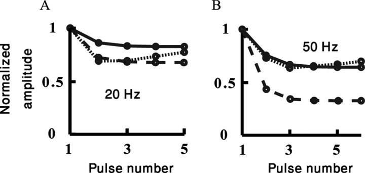
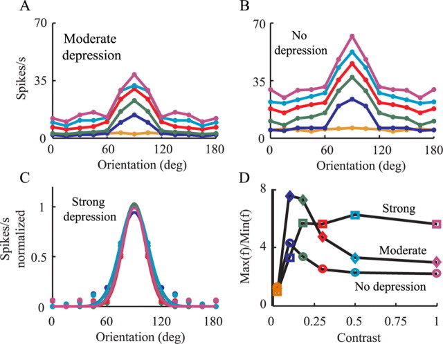
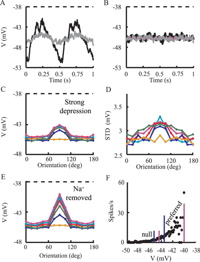
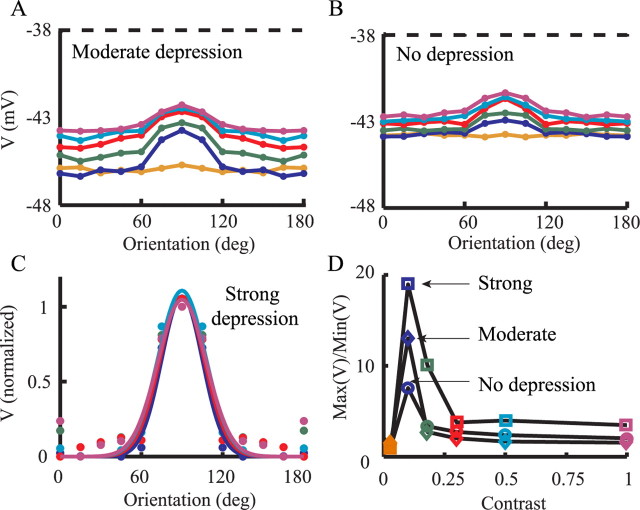
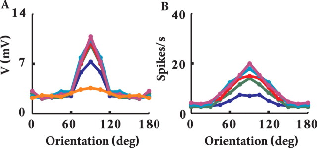
Simple cells in layer 4 of the primary visual cortex of the cat show contrast-invariant orientation tuning, in which the amplitude of the peak response is proportional to the stimulus contrast but the width of the tuning curve hardly changes with contrast. This study uses a detailed model of spiny stellate cells (SSCs) from cat area 17 to explain this property. The model integrates our experimental data, including morphological and intrinsic membrane properties and the number and spatial distribution of four major synaptic input sources of the SSC: the dorsal lateral geniculate nucleus (dLGN) and three cortical sources. The model also includes synaptic properties of these inputs. The cortical input served as sources of background activity, and visual stimuli was modeled as sinusoidal grating. For all contrasts, strong synaptic depression of the dLGN feedforward afferents compresses the firing rates in response to orthogonal stimuli, keeping these rates at practically the same low level. However, at preferred orientations, despite synaptic depression, firing rate changes as a function of contrast. Thus, when embedded in an active network, strong synaptic depression can explain contrast-invariant orientation tuning of simple cells. This is true also when the dLGN inputs are partially depressed as a result of their spontaneous activity and to some extent also when parameters were fitted to a more moderate level of synaptic depression. The model response is in close agreement with experimental results, in terms of both output spikes and membrane voltage (amplitude and fluctuations), with reasonable exceptions given that recurrent connections were not incorporated.

Figure 1.

Model overview: morphology of the modeled SSC and its synaptic input. The modeled L4 SSC is shown in the center with all ∼5500 synapses depicted in circles (many synapses overlap because of the segmentation in NEURON). In each of the four corners, the circles depicting the synapses from only one input source are superimposed on the SSC model, using the same color for a given input source (blue, inhibition; green, SSCs; yellow, dLGN; red, L6 input). For each input source, there is also a somatic voltage trace showing the short-term synaptic dynamics of this specific synapse. These traces were computed after the activation of a single axon from the corresponding input source. In this case, for all four input sources, the synapses belonging to a single axon contacted the dendritic tree at a distance of ∼50 μm from the soma and were activated at 40 Hz. Note the different number of synapses, amplitudes, and the short-term plasticity of each of the inputs. In the present study, all cortical input sources are activated for the purpose of generating realistic background activity for the modeled SSC, but there are no intracortical interactions.

Figure 2.

Comparison between in vitro recordings of SSCs (left column) and model response (right column). A, Response of an SSC to step current depolarization; B, response of the modeled SSC to step current injection. C, D, Adaptation of firing frequency in experiments versus model, correspondingly. Measured instantaneous firing frequencies are marked for three corresponding current injections denoted in insets. E, I/f curves at steady state for four different SSCs in experiments; F, model I/f curve at steady state. Data in A, C, and E are taken from the laboratory of Stratford et al. (unpublished results).

Figure 3.

Modeling the thalamic input. A, The modeled SSC with 360 synaptic contacts (90 axons) arising from the dLGN (each filled circle represents 4 dLGN contacts). B, Distribution of dLGN synaptic contacts as a function of distance from the soma. C, Strong short-term synaptic depression of the dLGN-to-SSC input. The amplitude of the second EPSP is shown as a function of the interpulse intervals (IPI) in a paired-pulse protocol. Model, Dashed line; experiment, continuous line (taken from Stratford et al., 1996). For large interpulse intervals, the second EPSP recovers from depression and attained the amplitude of the first EPSP of 1.35 mV. The inset shows the modeled short-term depression for a single dLGN input at interpulse intervals of 25 ms (40 Hz). D, Model firing output in response to random and asynchronous activation of all 90 dLGN afferents converging onto the modeled SSC; each dLGN afferent fires randomly at 20 Hz. Because there are only 360 dLGN synapses with a strong synaptic depression, only one spike is elicited in this case.

Figure 4.

Modeling dLGN response to visual input. A, Temporal waveform of firing rates of a dLGN afferent in response to drifting grating at 2 Hz at low contrast of 10% (thin line) and high contrast of 100% (thick line) (see Eq. 4 in Materials and Methods). Inset illustrates a grating stimulus, drifting at the indicated direction. Circles denote the center and surround RF of the dLGN afferent. Dashed line depicts the spontaneous firing rate of the dLGN axons (10 Hz). B, Contrast–response function, showing maximal dLGN response to six different contrasts (model was constructed to fit the results of Sclar, 1987) (see Materials and Methods).

Figure 5.

Firing response of modeled SSC to visual input. Firing rates in A–C are calculated by binning the output spike train to 40 ms bins and averaging over 60 cycles of 1 s each. A, Response rate for preferred stimulus at 10% contrast; B, response rate for preferred stimulus at 100% contrast. C, Response rate for orthogonal stimulus at 100% contrast. Insets illustrate stimuli drifting at indicated direction (arrow). Small circles depict the center of the RFs of 90 dLGN afferents. Red circles are OFF center RFs, whereas blue circles are ON center RFs. D, Tuning curve of the peak of the average response, for each orientation and for different contrasts at bins of 40 ms (from lower to upper curves, contrast is 3, 10, 18, 30, 50, and 100%). Note the emergence of tuning width contrast invariance.

Figure 6.

Fit of modeled dLGN-to-SSC depressing synapses to a train of stimuli. The amplitude of the nth EPSP in a train is shown as a function of the pulse number in the train at 20 Hz (A) and 50 Hz (B). Responses are normalized to the first EPSP amplitude. Dotted line, In vivo recordings, monosynaptic input (Boudreau and Ferster, 2005); continuous line, model with moderate depression; dashed line, model with strong depression. Note the similarities in depression for the 20 Hz and the differences in depression for the 50 Hz dLGN stimulation.

Figure 7.

Quantification of tuning curves of firing response to visual input. A, B, Firing response of modeled SSC for different contrasts (colors as in Fig. 5D) for moderate depression (A) and for the case without depression (B). C, Best Gaussian fits (continuous lines) to model response (circles) for the strong depression (same data as in Fig. 5D). D, The ratio between the maximal firing rate (at the preferred orientation) and the averaged firing rates for the four nonpreferred orientations (0, 15, 30, and 45°) is plotted against contrast, for the strong depression (squares), for the moderate depression (diamonds), and for the case without depression (circles).

Figure 8.

Membrane voltage responses to visual stimuli. A, Averaged voltage responses for preferred stimuli at contrast of 3% (gray line) and contrast of 100% (black line). Dashed line shows threshold for spike firing. B, Averaged voltage responses for orthogonal stimuli at contrast of 3% (gray) and contrast of 100% (black). Purple line shows average voltage without visual stimulus (background activity as described in Materials and Methods). C, Tuning curve for the peak averaged membrane potential for time bins of 40 ms. D, As in C but for the SD of the membrane potential. E, As in C but for a model without the sodium channels. F, V/f curve for the model. Blue lines (left and right) indicate the average membrane voltage for 10% contrast (at orthogonal and preferred orientations). Pink lines (left and right) indicate the average membrane voltage for 100% contrast (at orthogonal and preferred orientations, respectively).

Figure 9.

Quantification of tuning curves to visual input for the average membrane potential. A, B, Average voltage response of the modeled SSC for different contrasts, as in Figure 8C, but for moderate depression (A) and for the case without depression (B). The spike threshold is indicated by the dashed line. C, Best Gaussian fits (continuous lines) to average voltage response (open circles) for the strong depression (same data as in Fig. 8C). D, The ratio between the maximal firing rate (at the preferred orientation) and the averaged firing rates for the four nonpreferred orientations (0, 15, 30, and 45°) is plotted against contrast, for the strong depression (squares), for the moderate depression (diamonds), and for the case without depression (circles). For each level of depression, the ratios were calculated after shifting all voltage data points by the absolute value of the minimal voltage point obtained at the lowest contrast at the orthogonal orientation (such that for this point the value is now 0).

Figure 10.

Membrane voltage fluctuations and aspect ratio for the strong depression parameters. A, Tuning curve of the peak-to-peak fluctuations of the averaged voltage for different contrasts (colors as in Figs. 5–9). B, Tuning curve of the spikes for a model with subfield aspect ratio of 1.75. The tuning curve is broader than for an aspect ratio of 3.3 (as was used throughout), but it remains contrast invariant.

References

1. Abbott LF, Varela JA, Sen K, Nelson SB. Synaptic depression and cortical gain control. Science. 1997;275:220–224. - PubMed
1. Ahmed B, Anderson JC, Douglas RJ, Martin KA, Nelson JC. Polyneuronal innervation of spiny stellate neurons in cat visual cortex. J Comp Neurol. 1994;341:39–49. - PubMed
1. Ahmed B, Anderson JC, Martin KA, Nelson JC. Map of the synapses onto layer 4 basket cells of the primary visual cortex of the cat. J Comp Neurol. 1997;380:230–242. - PubMed
1. Ahmed B, Anderson JC, Douglas RJ, Martin KA, Whitteridge D. Estimates of the net excitatory currents evoked by visual stimulation of identified neurons in cat visual cortex. Cereb Cortex. 1998;8:462–476. - PubMed
1. Anderson JC, Douglas RJ, Martin KA, Nelson JC. Map of the synapses formed with the dendrites of spiny stellate neurons of cat visual cortex. J Comp Neurol. 1994a;341:25–38. - PubMed
Publication types
LinkOut - more resources