Extracting the hierarchical organization of complex systems

Abstract

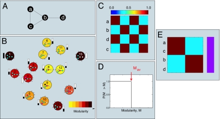
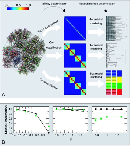
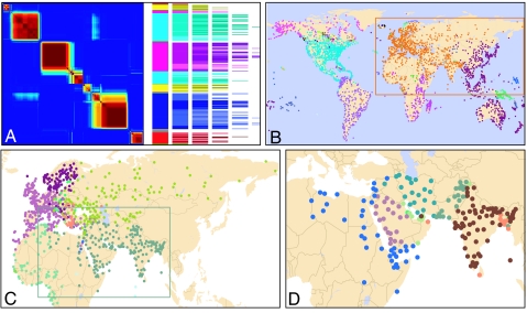
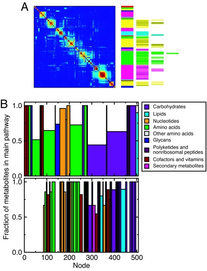
Extracting understanding from the growing "sea" of biological and socioeconomic data is one of the most pressing scientific challenges facing us. Here, we introduce and validate an unsupervised method for extracting the hierarchical organization of complex biological, social, and technological networks. We define an ensemble of hierarchically nested random graphs, which we use to validate the method. We then apply our method to real-world networks, including the air-transportation network, an electronic circuit, an e-mail exchange network, and metabolic networks. Our analysis of model and real networks demonstrates that our method extracts an accurate multiscale representation of a complex system.

Fig. 1.

Schematic illustration of our method for a simple network. (A) Example network. (B) Modularity landscape. For the example network, there are 15 distinct groupings of nodes into modules. Each large colored circle represents a partition, which we draw inside the circle, with different colors indicating different modules. For clarity, we label each partition with a number from 1 to 15. The color of the partition circle indicates the modularity of that partition following the color code on the bottom right-hand side of the diagram. For simplicity, we consider only single node changes; thus, we connect two partitions, for instance 1 and 2, because the change of a node to a new module in partition 1 generates partition 2. The arrows show the direction of increasing modularity. Local maxima correspond to those partitions that do not point to any other partition; that is, the change of a single node does not increase the modularity. In the example, there are two local maxima: partition 1 and partition 15. To illustrate the concept of basin of attraction, we show next to each partition a colored bar (black and white) that represents the probability that a walker that starts from, for instance, partition 2 and only moves to partitions with larger modularity ends up in either of the local maxima. We use white to indicate partition 15 and black to indicate partition 1. (C) Coclassification matrix. We show the number of times two nodes are classified in the same module, starting from a random partition. Note that nodes a, c and b, d are always classified together because they are in the same module in both local maxima (partitions 1 and 15). In contrast, nodes a and b are only in the same module for one of the maxima (partition 1); therefore, the coclassification is lower than one, but larger than zero. (D) Comparison with randomized networks. In this case, this is the only network that one can build keeping the same degree distribution and not allowing for self-loops. Therefore, the average modularity for the local maxima of the randomized networks and that of the network under analysis are the same. Thus, our conclusion is that this network has no internal organization. (E) Representation of the hierarchical organization for the example network. We show the ordered coclassification matrix on the Left, and on the Right is the tree showing the organization of the nodes into modules. In this case, the network has no significant structure; thus, we show a bar of a single color indicating that there is a single module. Note that a modularity maximization algorithm would have a certain chance (the probability depending on the specific algorithm) of finding partition 15 as the optimal partition and would thus conclude that the network does have a modular structure.

Fig. 2.

Affinity measures and clustering methods. (A) We generate a model network comprised of 640 nodes with average degree 16 and with a three-level hierarchical structure (see SI Fig. 8 for results for a network with a “flat” organization of the nodes). We show the affinity matrices A_ij obtained for two different measures: (i) topological overlap (11) and (ii) coclassification (see text and Supplementary Information). The color scale goes from red for an affinity of one to dark blue for an affinity of zero. At the far right, we show the hierarchical tree obtained by using two different methods: hierarchical clustering and the “box clustering” method we propose. In the hierarchical clustering tree, the vertical axis shows the average distance, d_ij = 1 − A_ij, of the matrix elements that have already merged. In the box-model clustering tree, each row corresponds to one hierarchical level. Different colors indicate different modules at that level. To better identify which are the submodules at a lower level, we color the nodes in the submodules with shades of the color used for the modules in the level above. Note that topological overlap fails to find any modular structure beyond a locally dense connectivity pattern. In contrast, the coclassification measure clearly reveals the hierarchical organization of the network by the “nested-box” pattern along the diagonal. Significantly, the hierarchical tree obtained via hierarchical clustering fails to reproduce the clear three-level hierarchical structure that the affinity matrix displays, whereas the box-model clustering tree accurately reproduces the three-level hierarchical organization of the network. (B) Accuracy of the method. We generate networks with 640 nodes and with built-in hierarchical structure comprising one (Left), two (Center), and three (Right) levels. The top level always comprises four modules of 160 nodes each. For networks with a second level, each of the top-level modules is organized into four submodules of 40 nodes. For the networks with three levels, each level-two module is further split into four submodules of 10 nodes. We build networks with different degrees of level cohesiveness by tuning a single parameter ρ (see SI Text). For low values of ρ, the levels are very cohesive, for high values of ρ the levels are weakly cohesive. Because we know a priori which are the nodes that should be coclassified at each level, we measure the accuracy as the mutual information between the empirical partition of the nodes and the theoretical one (23). We plot the mutual information versus ρ and, for comparison, we also plot the accuracy of a standard community detection algorithm (24) in finding the top level of the networks (dashed green line). Each point is the average over 10 different realizations of the network. Filled circles, empty squares, and filled diamonds represent the accuracy at the top, middle, and lowest levels, respectively. Note that our method is as good at detecting communities as a standard community detection algorithm for networks with a flat organization of the nodes. Additionally, our method is able to detect the top level for all cases analyzed, whereas standard modularity optimization algorithms are not.

Fig. 3.

Hierarchical organization of the air-transportation network. (A) Global-level affinity matrix and hierarchical tree (the representation is the same used in Fig. 2). (B) Top-level modules. Each dot represents a city and different colors represent different modules. Note that the top level in the hierarchy corresponds to major geopolitical units. (C) The “Eurasian” module (which is composed of the majority of European countries, ex-Soviet Union countries, Middle-Eastern countries, India, and countries in Northern half of Africa) splits for levels ℓ = 2 into five submodules. (D) The “Near and Middle East” submodule further splits into seven submodules for ℓ = 3 (D). Note that the air-transportation network is large and very dense (Table 1), and thus the organization of the network is not at all apparent (SI Fig. 11). Remarkably, the modules our method detects show a clear agreement with geopolitical units.

Fig. 4.

Hierarchical structure of metabolic networks. (A) Global-level affinity matrices and hierarchical trees for the UCSD reconstruction of the metabolic network of E. coli (43). The overall organization of the network is similar and independent of the reconstruction used to build the network (see SI Fig. 11). (B) We analyze the within-module consistency of metabolite pathway classification for the first (Upper plot) and the second (Lower plot) levels. For each module, we first identify the pathway classifications of the corresponding metabolites; then, we compute the fraction of metabolites that are classified in the most abundant pathway. In the plots, each bar represents one module, its width being proportional to the number of nodes it contains. We color each bar according to its most abundant pathway following the color code on the right-hand side. At the second level (Lower plot), we show each submodule directly below its corresponding top level module. Again, the width of each submodule is proportional to its size. Note that, at the first level (Upper), for all modules except one, the most abundant pathway is composed of more than 50% of the metabolites in the module. Remarkably, at the second level (Lower), for most of the modules all of the metabolites are classified in the same pathway. Moreover, at the second level, we detect smaller pathways that are not visible at the top level.

References

1. Pennisi E. Science. 2005;309:94. - PubMed
1. Oltvai ZN, Barabási A-L. Science. 2002;298:763–764. - PubMed
1. Alon U. Science. 2003;301:1866–1867. - PubMed
1. Itzkovitz S, Levitt R, Kashtan N, Milo R, Itzkovitz M, Alon U. Phys Rev E. 2005;71 016127. - PubMed
1. Arenas A, Díaz-Guilera A, Pérez-Vicente CJ. Phys Rev Lett. 2006;96:114102. - PubMed
Publication types
LinkOut - more resources