Fast, comprehensive two-dimensional liquid chromatography

Abstract

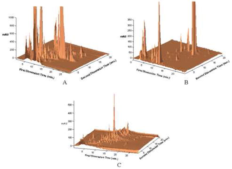
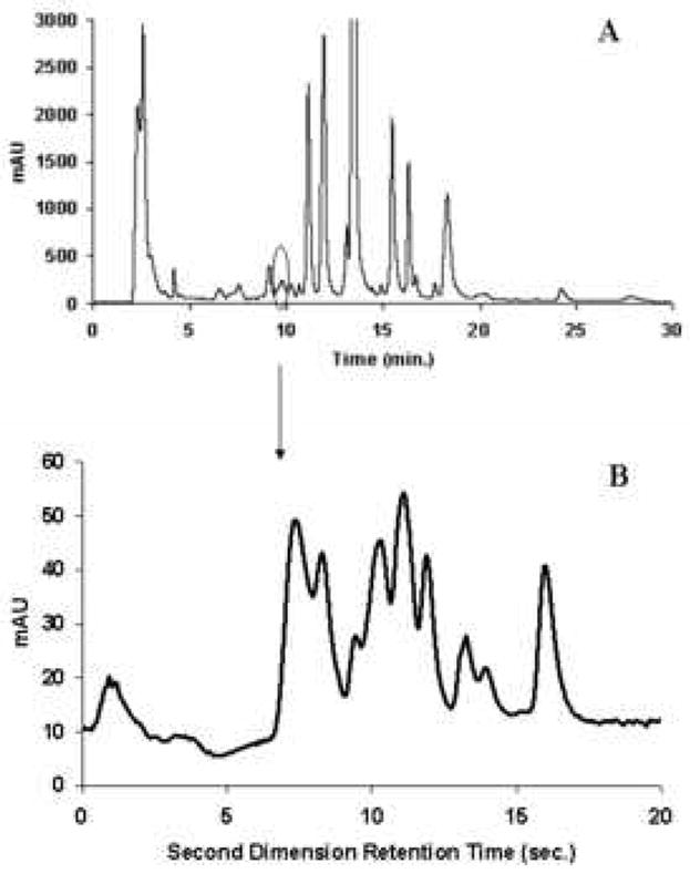
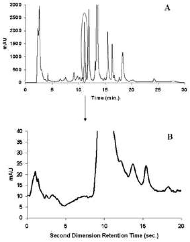
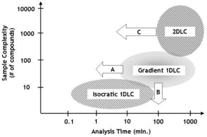
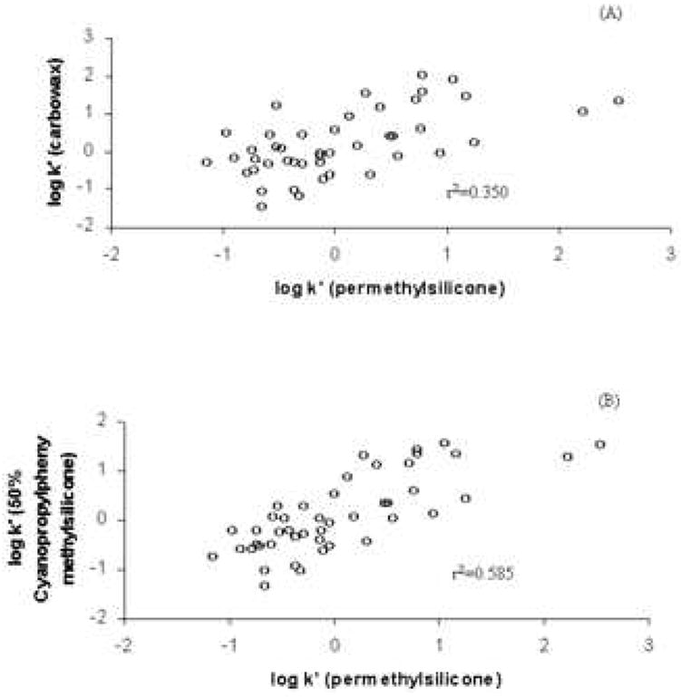
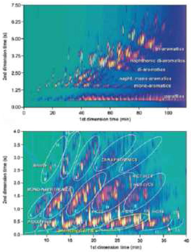
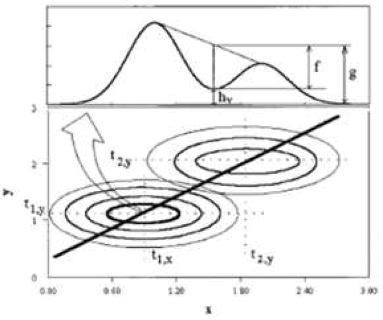
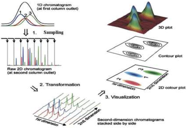
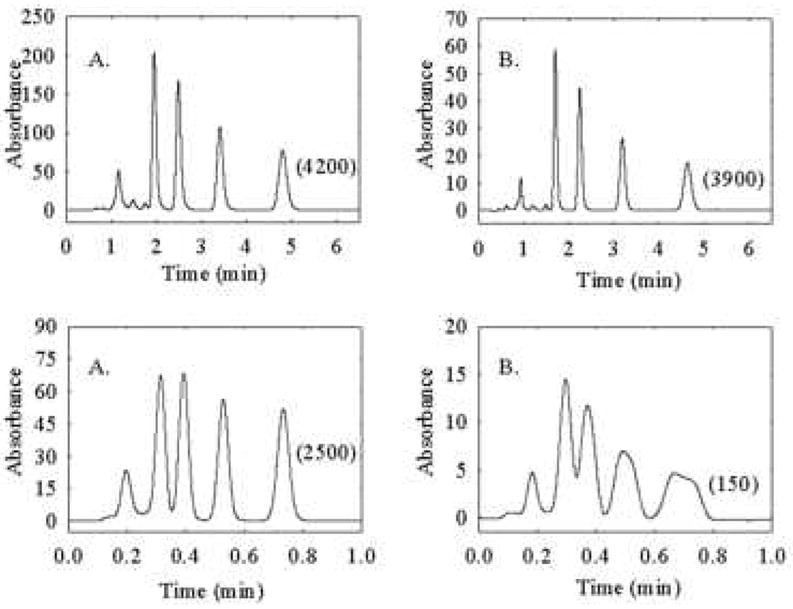
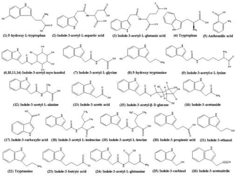
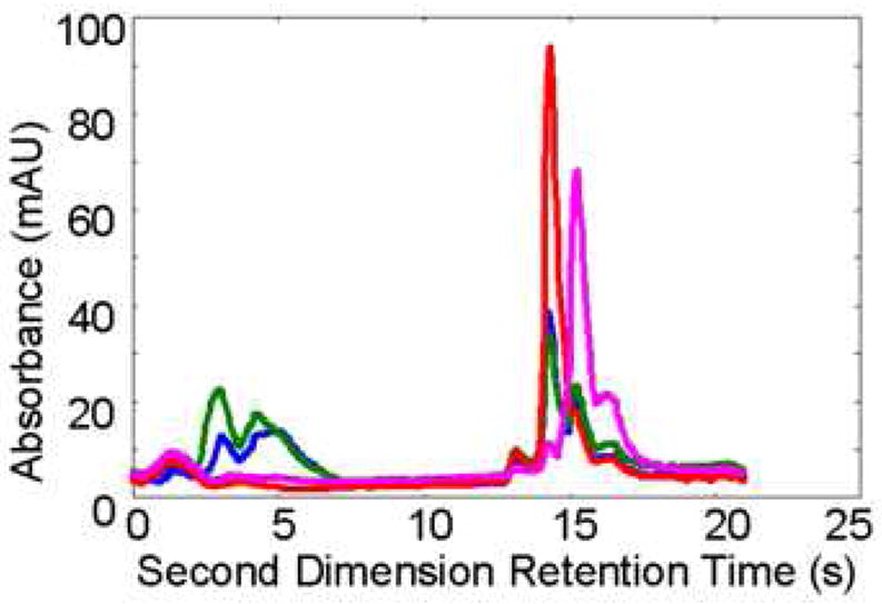
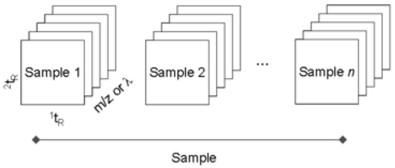
The absolute need to improve the separating power of liquid chromatography, especially for multi-constituent biological samples, is becoming increasingly evident. In response, over the past few years, there has been a great deal of interest in the development of two-dimensional liquid chromatography (2DLC). Just as 1DLC is preferred to 1DGC based on its compatibility with biological materials we believe that ultimately 2DLC will be preferred to the much more highly developed 2DGC for such samples. The huge advantage of 2D chromatographic techniques over 1D methods is inherent in the tremendous potential increase in peak capacity (resolving power). This is especially true of comprehensive 2D chromatography wherein it is possible, under ideal conditions, to obtain a total peak capacity equal to the product of the peak capacities of the first and second dimension separations. However, the very long timescale (typically several hours to tens of hours) of comprehensive 2DLC is clearly its chief drawback. Recent advances in the use of higher temperatures to speed up isocratic and gradient elution liquid chromatography have been used to decrease the time needed to do the second dimension LC separation of 2DLC to about 20s for a full gradient elution run. Thus, fast, high temperature LC is becoming a very promising technique. Peak capacities of over 2000 and rates of peak capacity production of nearly 1 peak/s have been achieved. In consequence, many real samples showing more than 200 peaks with signal to noise ratios of better than 10:1 have been run in total times of under 30 min. This report is not intended to be a comprehensive review of 2DLC, but is deliberately focused on the issues involved in doing fast 2DLC by means of elevating the column temperature; however, many issues of broader applicability will be discussed.

Figure 1

Block diagram of instrumentation for 2DLC. The dashed box indicates that the second dimension of the system effectively acts as a chemically selective detector for the peaks that elute from the first dimension column.

Figure 2

Illustration of the multiplicative relationship between the peak capacities of the independent first and second dimensions in comprehensive two-dimensional separations.

Figure 3

Schematic of instrumentation used for comprehensive, fast 2DLC using high temperature and high velocity to achieve high speed. From ref. [10].

Figure 4

Comparison of (A) Jorgenson et al.’s 2D- and (B) Carr et al.’s 2D-separation chromatograms. Conditions: (A) protein sample, 5 μL/min, 0% to 100% buffer B from 20 to 260 mins; buffer A, 0.2 M NaH₂PO₄, pH 5; buffer B, 0.2 M NaH₂PO₄/0.25 M Na₂SO₄, pH 5. Detection at 215 nm. (B) corn seedling extract, First Dimension, 50 mm × 2.1 mm i.d. Discovery HS-F5; 0.10 mL/min; 5 to 70% B from 0 to 23 mins; buffer A, 20 mM NaH₂PO₄, 20 mM NaClO₄, pH 5.7; solvent B, acetonitrile; 40 °C; Second Dimension, 50 mm × 2.1 mm i.d. ZirChrom-CARB; 3.00 mL/min; 0 to 70% B in 17.4 s; buffer A, 20 mM HClO₄ in water; solvent B, acetonitrile; 110 °C; detection at 220 nm. Fig. 3(A) from ref. [6], fig 3(B) from ref. [10]. Note the huge differences in times scales in A and B.

Figure 5

2DLC chromatograms of (A) urine; (B) coffee; (C) red wine. Conditions: Second Dimension – Flow rate, 3.00 mL/min.; Gradient elution from 0-85 %B from 0-21 seconds, where A is 10 mM perchloric acid in water, and B is acetonitrile; injection volume, 34 μL, Temperature, 110 °C, 33 mm × 2.1 mm i.d. ZirChrom-CARB (8% carbon (w/w)). First Dimension-, Urine - Flow rate, 0.10 mL/min.; Gradient elution from 0-50 %B from 0-30 minutes, where A is 20 mM sodium dihydrogen phosphate, 20 mM sodium perchlorate, pH 5.7, and B is acetonitrile ; injection volume, 20 μL, Temperature, 35 °C, 200 mm × 2.1 mm i.d. Discovery HS-F5; Coffee - Flow rate, 0.10 mL/min.; Gradient elution from 0-40 %B from 0-30 minutes, where A is 20 mM sodium dihydrogen phosphate, 20 mM sodium perchlorate, pH 5.7, and B is acetonitrile ; injection volume, 20 μL, Temperature, 35 °C, 100 mm × 2.1 mm i.d. Discovery HS-F5; Red Wine - Flow rate, 0.10 mL/min.; Gradient elution from 0-50 %B from 0-23 minutes, where A is 20 mM sodium dihydrogen phosphate, 20 mM sodium perchlorate, 0.2 mM EDTA, pH 5.7, and B is acetonitrile ; injection volume, 20 μL, Temperature, 35 °C, 100 mm × 2.1 mm i.d. Discovery HS-F5. From ref. [11].

Figure 6

First (A) and second (B) dimension chromatograms of corn seedling separation in Fig. 4A, where the second dimension chromatogram is obtained from 9.80-10.15 min in the first dimension From ref. [10].

Figure 7

First and second dimension chromatograms of corn seedling separation in Fig. 4A, where the second dimension chromatogram is obtained from 11.55-11.90 min in the first dimension. From ref. [10].

Figure 8

Domain of various LC modes as a function of sample complexity and analysis time. The elipses indicate the historical domains of the different modes; the arrows indicate changes in the perceived limits of these domains as a result of recent fundamental research in these areas.

Figure 9

(A) Plot of log k’ vs. log k’ of carbowax and permethylsilicone phases, (B) Plot of log k’ vs. log k’ of 50% cyanopropylphenyl methylsilicone and permethylsilicone phases. Both show a significant lack of orthogonality. Data re-plotted from ref. [38].

Figure 10

2DGC chromatogram of a light cycle oil using a (25 m × 0.25 mm DB-1) × (1.5 m × 0.1 mm OV-1701) column combination (top), and a non-aromatic hydrocarbon solvent using a (10 m × 0.25 mm CP Sil-2 CB) × (2.5 m × 0.1 mm BPX-50) column combination (bottom). 1 through 13: alkanes; 1: branched C₁₀s; 2: n-C₁₀, 3: branched C₁₁s; 4: n-C₁₁, 5: branched C₁₂s; 6: n-C₁₂; 7: branched C₁₃s; 8: n-C₁₃; 9: branched C₁₄s; 10: n-C₁₄; 11: branched C₁₅s; 12: n-C₁₅; 13: branched C₁₆s; 14: unknown; 15: trans-decalin; 16: cis-decalin;17: trans-methyl-decalins; 18: cis-methyl-decalins; A through E: mono-naphthenes C₁₀ through C₁₄; F through J: di-naphthenes C₁₀ through C₁₃. From ref. [40].

Figure 11

Schematic representation of the two-dimensional resolution measurement using a 2D contour (bottom) and the corresponding slice for resolution determination. From ref. [58].

Figure 12

Diagram of the flow of information as it is collected and analyzed in a comprehensive 2D separation experiment. Step 1 shows that the collection and transfer of aliquots of first dimension column effluent and subsequent separation in the second dimension column produces a series of sequential second dimension chromatograms collected as one string of data. Steps 2 and 3 show how the sequential second dimension chromatograms can be reshaped to produce a variety of different representations of the 2D chromatogram. Adapted from ref. [16].

Figure 13

Simulated demonstration of the effect of the first dimension sampling time (t_s) on the first dimension peak capacity. Simulated condition: first dimension peak standard deviation before sampling is 0.25 min, second dimension peak standard deviation is 0.25 sec, the first dimension retention times are 4, 6, 7 min, the second dimension retention times are 5, 5, 5 sec, peak heights are uniform. Note that as t_s increases one first sees a loss in the more poorly resolved peak and then a loss in the better resolved peak.

Figure 14

Quantity σ_s/σ as a function of N. (A) sampling is 4σ/N prior to t₀ = t̄ – 4σ; (B) the average σs/σ; (C) sampling is 2σ/N prior to t₀ = t̄ – 4σ; (D) sampling is in phase (starts at t₀ = t̄ – 4σ). From ref. [58].

Figure 15

Effect of slow first dimension sampling compared to first dimension peak width on first dimension peak capacity. The ideal first dimension peak capacity (——) is calculated for a diverse mixture of peptides using the method of Wang et al. [66] at 40 °C and assumes no effect of undersampling. The other three curves are calculated by simply dividing the analysis time by the sampling time (t_s).

Figure 16

Demonstration of the weakness of the correlation coefficient as a metric of separation space utilization in 2DLC systems.

Figure 17

The geometric orthogonality concept. Hypothetical separation of 100 analytes in a 10 × 10 normalized separation space. (A) Nonorthogonal system, 10% area coverage represents 0% orthogonality. (B) Hypothetical ordered system, full area coverage. (C) Random, ideally orthogonal, system, area coverage is 63% representing the 100% orthogonality. From ref. [73].

Figure 18

Correlation of (A) peak capacity calculated via Eq. 9 and (B) peak capacity calculated via Eqn. 8 with average resolution of eleven peptides. Each point represents one of the 2651 conditions generated in Monte Carlo simulation. The linear regression lines are also displayed. From ref. [66].

Figure 19

Effect of gradient time on peak capacity of eleven peptides at various flow rates. From ref. [66].

Figure 20

Effect of flow rate on peak capacity of eleven peptides at various gradient times. From ref. [66].

Figure 21

Effect of temperature on peak capacity of eleven peptides at two flow rates. From ref. [66].

Figure 22

Effect of temperature on peak capacity of eleven peptides in three cases. Case a: ϕ_f is kept constant at 0.409 (– –); Case b: ϕ_f is optimized by Solver to maximize peak capacity (—); Case c: Both ϕ_f and flow rate are simultaneously optimized by Solver to maximize peak capacity (----). From ref. [66].

Figure 23

Isocratic Poppe plot for packed bed columns with different particle sizes. Conditions: ΔP = 400 bar, T = 40 °C, ϕ = 500, η = 0.69 cPoise, D_m = 1 × 10^-5 cm²/sec. Coefficients in reduced van Deemter equation were measured on a 50 × 2.1 mm 3.5 μm Zorbax SB-C18 column using heptanophenone in 40 % acetonitrile (v/v) at 40 °C (k’ = 20): A = 1.04, B = 15.98, C = 0.033. Each dotted line represents a constant column dead time. From ref. [105].

Figure 24

Effect of particle size on gradient elution Poppe plots. Sample was a mixture of eleven representative peptides. Conditions: ΔP = 400 bar, T = 40 °C, ϕ = 500, η = 0.69 cPoise. Diffusion coefficients of the peptides were estimated using the Wilke-Chang equation. Coefficients of the reduced van Deemter equation were measured on a 50 × 2.1 mm 3.5 μm Zorbax SB-C18 column using heptanophenone in 40 % acetonitrile (v/v) at 40 °C (k’ = 20): A = 1.04, B = 15.98, C = 0.033. Open triangles represent the points where the column length is 1.0 cm and open circles represent the points where the flow rate is at 5.0 mL/min. Each dotted line represents a constant gradient time. From ref. [105].

Figure 25

Effect of operating temperature and maximum pressure drop with 2 μm particles on gradient Popple plots for packed beds. Curve a: T = 40 °C, ΔP = 400 bar (normal temperature and typical maximum pressure). Curve b: T = 100 °C, ΔP = 400 bar. Curve c: T = 40 °C, ΔP = 1000 bar. Other conditions are the same as Fig. 19. From ref. [105].

Figure 26

Effect of mobile phase composition and temperature on viscosity. Experimental data and fitted curves for the viscosity of (A) acetonitrile/water, (B) methanol/water mixtures at different temperatures. Symbols, temperature (°C, top to bottom): 15; 20; 25; 30; 35; 40; 45; 50; 55; 60. From ref. [109].

Figure 27

Theoretical effect of temperature on a plot of HETP vs. linear velocity. Conditions: The particle diameter is taken as 3 μm and the reduced linear velocity is based on diffusion at a fixed temperature ((D_m at 25 °C = 6*10^-7 cm²/s). The linear velocity (u) is increased and the reduced plate height is calculated from a modified Knox equation: $\mathrm{h}=\mathrm{A}+\frac{\mathrm{B}}{\mathrm{\nu }}+\mathrm{C}\mathrm{\nu }+\mathrm{D}{\mathrm{\nu }}^{2/3}+\frac{3{\mathrm{D}}_{\mathrm{m}}}{8{\mathrm{k}}_{\mathrm{d}}{\mathrm{d}}_{\mathrm{p}}^2}\mathrm{\nu }(\mathrm{A}=1.5,\mathrm{B}=0.8,\mathrm{C}=0.3,\mathrm{D}=0.04)$ at each velocity and temperature. Fast desorption kinetics are assumed (E_a = 20 kJ/mol, k_o = 1*10¹³s). From ref. [97].

Figure 28

Experimental effect of temperature on column dynamics. Conditions: 25 °C (decanophenone, k’ = 12.2);, 80 °C (dodecanophenone, k’ = 7.39);, 120 °C (tetradecanophenone, k’ = 12.3);, 150 °C (tetradecanophenone, k’ = 7.00). From ref. [109].

Figure 29

Effect of column diameter on thermal mismatch broadening. Top chromatograms for (A) 2.1 mm i.d. × 50 mm and (B) 4.6 mm i.d. × 50 mm columns. The columns were thermostated at 27 °C and the column linear velocity is 0.25 cm/s. Bottom chromatograms show the effect of temperature mismatch broadening on peak shape as a function of column diameter at elevated temperature. Column linear velocity is 1.75 cm/s. Preheater (5 cm × 0.005-in. i.d.) and column are in a stirred oil bath at 60 °C. Mobile-phase compositions were adjusted to 55:45 and 60:40 acetonitrile/water (v/v) for the narrow- and conventional-bore columns, respectively. Solutes are (1) toluene, (2) ethylbenzene, (3) propylbenzene, and (4) butylbenzene. Numbers in parentheses are the efficiencies of butylbenzene. From ref. [99].

Figure 30

Structures of twenty six metabolites of indole-3-acetic acid. Compounds 6,10,11, and 14 are all structural isomers of indole-3-acetyl-myoinositol. The diversity of chemical functionality encountered in studies of these kinds of molecules (i.e., metabolomics) makes 2D method development considerably more challenging than in proteomics. From ref. [10].

Figure 31

Second dimension chromatogram at 2.8 min for mutant corn extract, monitored at four different wavelengths, 201 nm (blue), 213 nm (green), 255 nm (red), and 315 nm (pink).

Figure 32

Data structure for 2D chromatographic data. The data dimensions include first and second dimension retention times and may include spectral information (m/z or wavelength) and/or sample number or concentration.

Figure 33

Demonstration of the ability of the PARAFAC method to find overlapped constituents in a 2D chromatogram. (a) First dimension separation of a corn seedling extract; (b) second dimension chromatogram; (c) contour plot of the data after two-dimensional separation; and (d) resolved constituent profiles after PARAFAC analysis.

Figure 34

Seven spectra chosen from the 95 constituents resolved from the corn seedling data set. These seven spectra are the most dissimilar found in the sample set.

Figure 35

Various spectra taken from the set of 95 spectra resolved from the corn data illustrating the differences and near identity of some of the spectra.

Figure 36

Comparison of chromatograms at 220 nm of the selected section of corn data from ref.[196]. (a) raw data; and (b) PARAFAC fitting results with background constituents omitted.

Figure 37

All peaks resolved by the PARAFAC algorithms. Blue – mutant only; green – wild type only; red – standard only; cyan – mutant and wild type; magenta – mutant and standard; yellow – wild type and standard; black – mutant, wild type, and standard. From ref. [196].

References

1. Karger BL, Snyder LR, Horvath C. An Introduction to Separation Science. John Wiley and Sons; New York: 1973.
1. Giddings JC. Anal Chem. 1984;56:1258A. - PubMed
1. Guiochon G, Beaver LA, Gonnord MF, Siouffi AM, Zakaria M. J Chromatogr. 1983;255:415.
1. Schure MR. In: Multidimensional Liquid Chromatography: Theory, Instrumentation and Applications. Cohen SA, Schure MR, editors. Wiley; New York: 2008.
1. Erni F, Frei RW. J Chromatogr. 1978;149:561.
Publication types