Auditory cortical receptive fields: stable entities with plastic abilities

Abstract

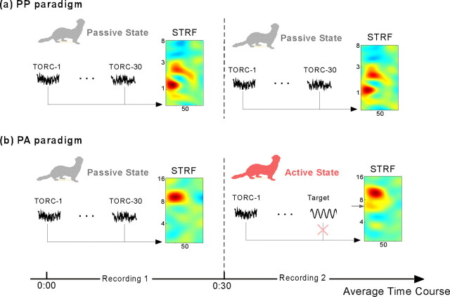
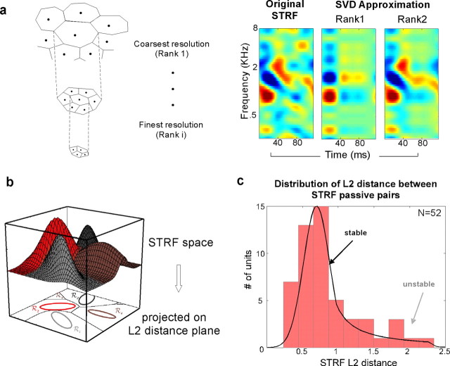
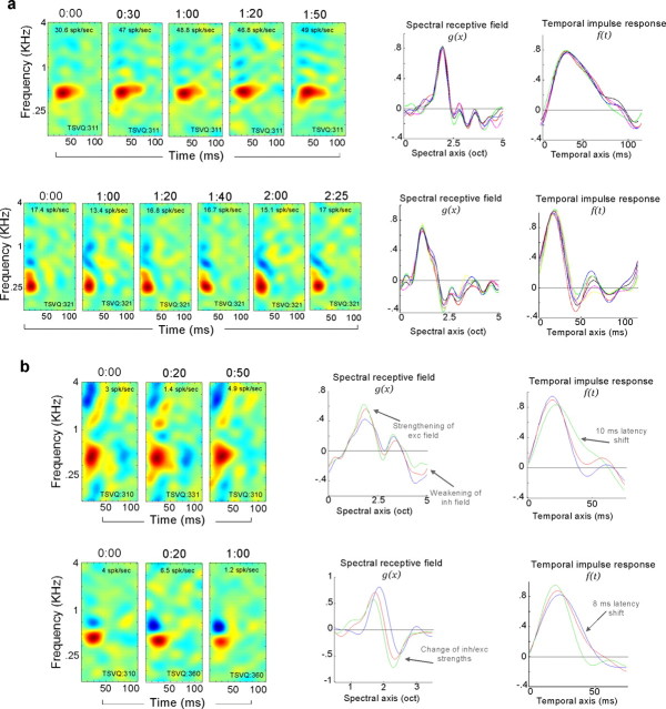
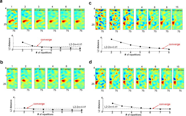
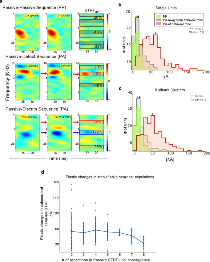
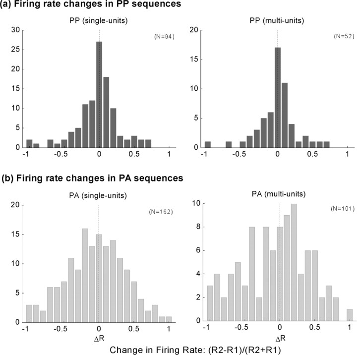
To form a reliable, consistent, and accurate representation of the acoustic scene, a reasonable conjecture is that cortical neurons maintain stable receptive fields after an early period of developmental plasticity. However, recent studies suggest that cortical neurons can be modified throughout adulthood and may change their response properties quite rapidly to reflect changing behavioral salience of certain sensory features. Because claims of adaptive receptive field plasticity could be confounded by intrinsic, labile properties of receptive fields themselves, we sought to gauge spontaneous changes in the responses of auditory cortical neurons. In the present study, we examined changes in a series of spectrotemporal receptive fields (STRFs) gathered from single neurons in successive recordings obtained over time scales of 30-120 min in primary auditory cortex (A1) in the quiescent, awake ferret. We used a global analysis of STRF shape based on a large database of A1 receptive fields. By clustering this STRF space in a data-driven manner, STRF sequences could be classified as stable or labile. We found that >73% of A1 neurons exhibited stable receptive field attributes over these time scales. In addition, we found that the extent of intrinsic variation in STRFs during the quiescent state was insignificant compared with behaviorally induced STRF changes observed during performance of spectral auditory tasks. Our results confirm that task-related changes induced by attentional focus on specific acoustic features were indeed confined to behaviorally salient acoustic cues and could be convincingly attributed to learning-induced plasticity when compared with "spontaneous" receptive field variability.

Figure 1.

Experimental design for PP and PA paradigms. a, PP paradigm. Sequences of receptive field recordings were performed in awake, nonbehaving animals (P). The stimulus set consisted of broadband noise-like stimuli known as TORCs, which were used to derive the spectrotemporal receptive field of each neuron using standard reverse correlation techniques. The successive recordings were performed over the course of 30 min to 2 h. b, PA paradigm. Similar receptive field sequences were measured using the same stimulus design but changing the behavioral state of the animal. Initially, a P receptive field was obtained from a nonbehaving animal. Next, the animal was engaged in a behavioral task (A) and a similar receptive recording was obtained again. The behavioral paradigm has been described previously (Fritz et al., 2003, 2005) and included the use of a set of TORC and single tone stimuli. Only the TORC stimuli were used for deriving the receptive fields in the active state, allowing us to compare receptive fields that are obtained from the same stimulus set but under different behavioral conditions.

Figure 2.

Stability analysis for receptive fields based on TSVQ. a, TSVQ analysis. Tree-structure vector quantization is a hierarchical clustering algorithm that organizes data at increasing levels of resolution (based on multiple scales). The right panel depicts the multiple resolutions of analysis used to cluster the STRF space. Each original receptive field matrix can be approximated by STRFs with different ranks using SVD. Each additional rank captures more specific features of the STRF. The rank-1 STRF fails to capture the orientation of the STRF and rather denotes the general tuning of the receptive field. By adding an additional degree (Rank-2), the original receptive field is now better approximated as an oriented function. b, Schematic of TSVQ clustering of STRF space [reproduced from Duda et al. (2001)]. Functions in the STRF space are projected on a two-dimensional plane by computing Euclidian distance (L2) between each pair. STRFs that have smaller L2 distances are deemed closer, and effectively belonging to a same cluster, and vice versa. c, Distribution of L2 distances in PP pairs. On average, most STRF pairs in the PP sequences tend to have a small L2 distance, making them effectively stable receptive fields (based on our stability criterion). The distribution, however, has a longer tail, indicating that a smaller subset of cells does in fact exhibit a wider variation in receptive field shapes over successive recordings.

Figure 3.

Clustering of receptive field space. The tree-structured diagram depicts the classification of STRFs at different levels of resolution. The gray versus green vertical branches illustrate a natural division of receptive fields into excitatory versus inhibitory units. The vertical direction reveals a more refined division of each branch by adding increasingly more information going from levels 1 to 4 (see description in Materials and Methods).

Figure 4.

Examples of stable versus labile units. a, Stable units. Each row shows a sequence of receptive fields obtained from successive recordings over the course of 2–2.5 h. The receptive fields show a remarkable stability and hardly change their main tuning features. The right panels depict the spectral receptive fields and temporal impulse responses extracted from these receptive fields and confirm the stability of the shape and tuning of the response properties of these units. The number shown on top of each STRF plot indicates the average firing rate of the cell during that particular recording. The L2 distances between the consecutive STRFs in the top example are 0.51, 0.52, 0.65, and 0.72 and in the second example are 0.38, 0.26, 0.35, 0.37, and 0.3. b, Labile units. The panels show examples of two labile units. The receptive fields obtained over the course of 1 h exhibit changes in the spectral and temporal tuning, as depicted in the right panels. The L2 distances between the consecutive STRFs in the first labile example are 0.94 and 1.05 and in the second labile example are 0.93 and 0.94.

Figure 5.

Convergence of receptive field estimates over time. Examples in a and b depict two units with rapidly converging STRFs. The top panels show the STRF estimate after increasing numbers of repetitions of the stimulus sequence (1, 2, up to 8 repetitions). The plot below the STRFs measures the L2 distance between every receptive field and its previous estimate. Examples in c and d illustrate two cases of slowly converging receptive fields. As reflected in the L2 distance plots, the STRFs keep changing after each repetition of the stimulus and take approximately six and seven stimulus iterations before reaching the convergence criterion.

Figure 6.

Local spectral changes in receptive fields in both behavioral and passive conditions. a, STRF sequences and difference in one PP and two PA examples. Each row depicts a sequence of two consecutive STRF measurements. The third panel shows the difference in STRF obtained by subtracting the second receptive field from the first one. The highlighted spectral bands in the STRF_diff illustrate the amount of change (ΔA) at that given band. b, Local spectral change in PP and PA populations in single units and multiunit clusters. Each panel shows the distribution of ΔA values at spectral bands across the tonotopic axis in passive STRF sequences in green, away from any behaviorally relevant spectral bands in gray (in PA sequences), and at the behavior tone in red (in PA sequences). The summary histograms (shown as smooth curves) depict a Gaussian curve to the underlying distributions. They reveal a significant difference between the three populations, with a mean value of 10.73% for PP and 17.74% for nonbehavioral bands in PA, in contrast with 53.14% for the behaviorally relevant tone locations. The same trend holds for multiunit data, with mean values of 10.59% for PP, 15.73% for nonbehavioral bands in PA, and 50.82% for behavioral bands.

Figure 7.

Change in firing rate in PP versus PA sequences. Each panel shows the distribution of rate changes in each sequence, measured as (R2 − R1)/(R2 + R1), where R1 is the average firing rate for the first measurement in a sequence, and R2 is the rate in the second measurement. The histograms reveal that that gain changes in both PP and PA cases are mostly symmetrical at ∼0. The main difference between the two cases is the noticeable increased variability in the PA recordings, possibly because of the changed attentional state, alertness level, and behavioral demands in the active condition.

References

1. Abut H. Vector quantization. Piscataway, NJ: IEEE; 1990.
1. Aertsen A, Johannesma P. The spectro-temporal receptive field: a functional characteristic of auditory neurons. Biol Cybernetics. 1981;42:133–143. - PubMed
1. Bair W. Visual receptive field organization. Curr Opin Neurobiol. 2005;15:459–464. - PubMed
1. Bar-Yosef O, Rotman Y, Nelken I. Responses of neurons in cat primary auditory cortex to bird chirps: effects of temporal and spectral context. J Neurosci. 2002;22:8619–8632. - PMC - PubMed
1. Breiman L, Friedman JH, Olshen RA, Stone CJ. Classification and regression trees. Boca Raton, FL: Chapman & Hall/CRC; 1984.
Publication types
LinkOut - more resources