Complete pattern of ocular dominance columns in human primary visual cortex

Abstract

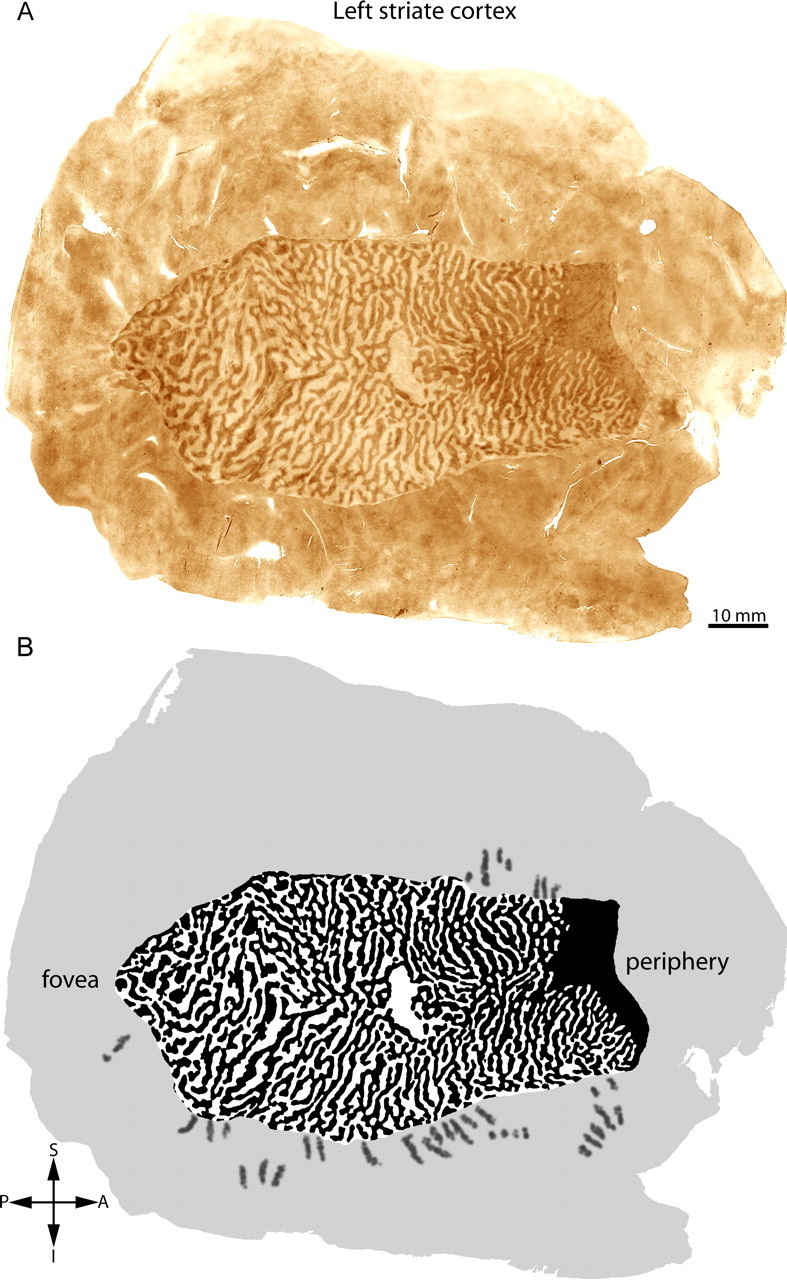
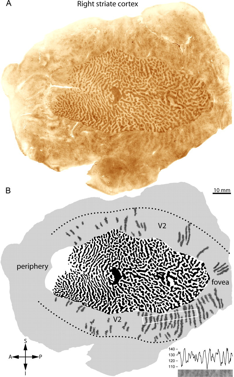
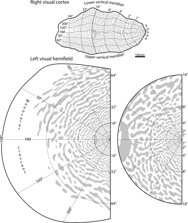
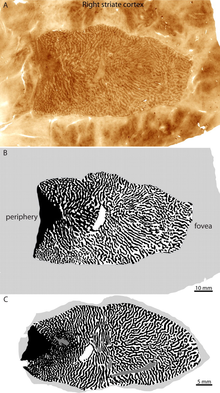
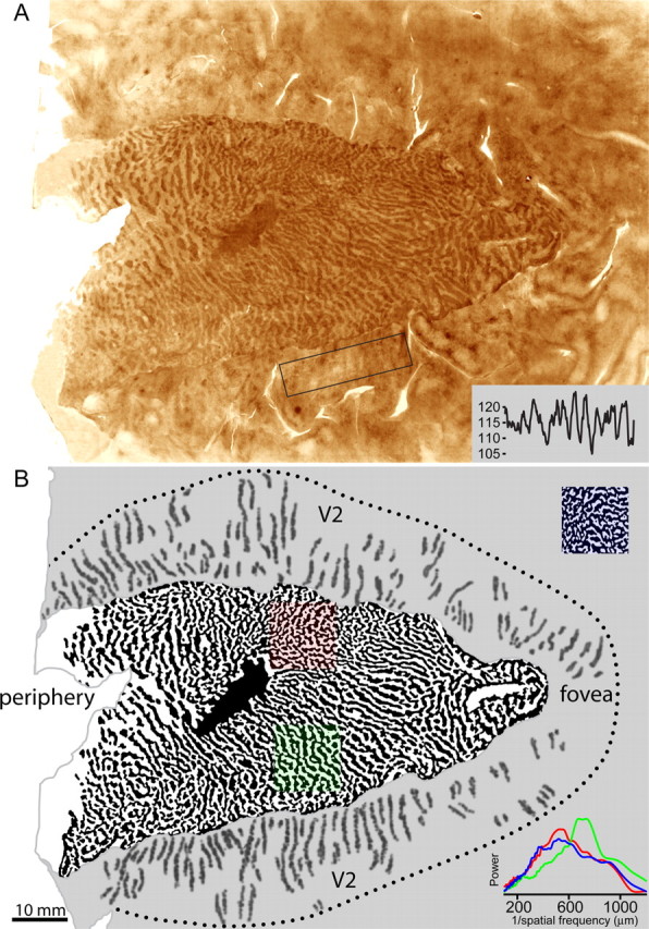
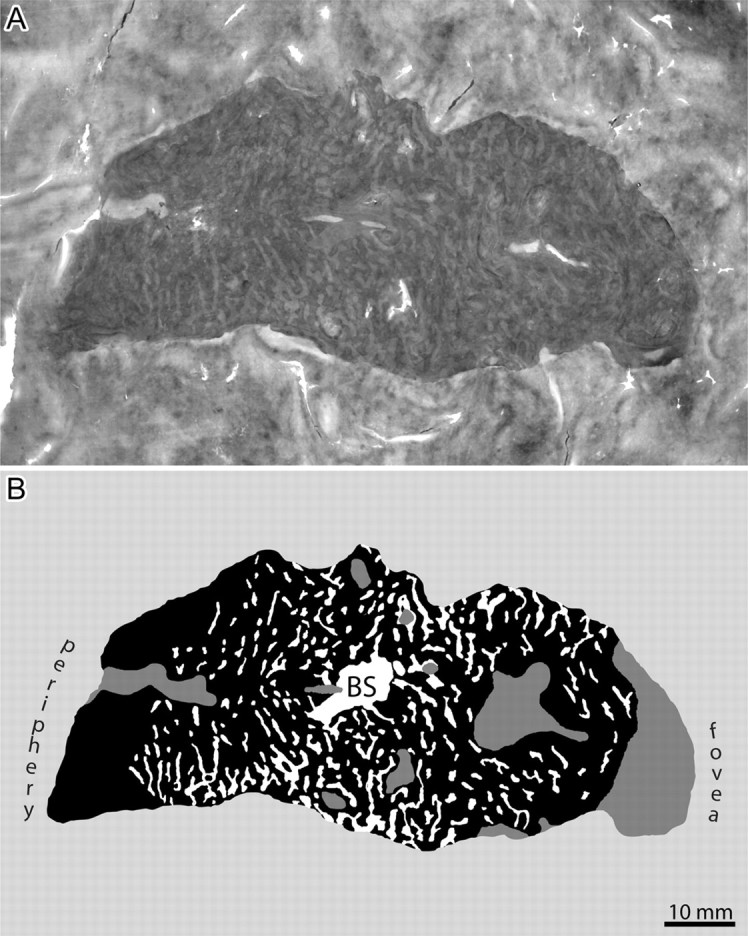
The occipital lobes were obtained after death from six adult subjects with monocular visual loss. Flat-mounts were processed for cytochrome oxidase (CO) to reveal metabolic activity in the primary (V1) and secondary (V2) visual cortices. Mean V1 surface area was 2643 mm2 (range, 1986-3477 mm2). Ocular dominance columns were present in all cases, having a mean width of 863 microm. There were 78-126 column pairs along the V1 perimeter. Human column patterns were highly variable, but in at least one person they resembled a scaled-up version of macaque columns. CO patches in the upper layers were centered on ocular dominance columns in layer 4C, with one exception. In this individual, the columns in a local area resembled those present in the squirrel monkey, and no evidence was found for column/patch alignment. In every subject, the blind spot of the contralateral eye was conspicuous as an oval region without ocular dominance columns. It provided a precise landmark for delineating the central 15 degrees of the visual field. A mean of 53.1% of striate cortex was devoted to the representation of the central 15 degrees. This fraction was less than the proportion of striate cortex allocated to the representation of the central 15 degrees in the macaque. Within the central 15 degrees, each eye occupied an equal territory. Beyond this eccentricity, the contralateral eye predominated, occupying 63% of the cortex. In one subject, monocular visual loss began at age 4 months, causing shrinkage of ocular dominance columns. In V2, which had a larger surface area than V1, CO stripes were present but could not be classified as thick or thin.

Figure 1.

Preparation of flat-mounts from the human occipital lobe. A, Intact right occipital lobe from case 2, after removal of the leptomeninges, showing the medial face. The dashed line indicates the V1/V2 border, where it is visible on the surface of the brain. Arrow, Parieto-occipital sulcus. cc, Splenium of corpus callosum; cs, calcarine sulcus. B, Midway through the dissection, showing the opened calcarine sulcus. The numbers denote corresponding locations in each image. C, Final flattened tissue block, ready to be frozen and cut with a microtome. The location of V1, determined later from CO-stained sections, is shown by the dashed line.

Figure 2.

The complete pattern of ocular dominance columns in the human brain. A, CO activity in layer 4Cβ montage of the left primary visual cortex after loss of the left eye in case 2. The CO pattern in V2 is a montage compiled from three sections passing through layer 4. The total area of the flat-mount is 10,117 mm². B, Ocular dominance columns rendered by high-pass Fourier filtering of the image in A, followed by application of a threshold function (see Materials and Methods). Columns are absent in the blind spot and monocular crescent regions. S, Superior; A, anterior; I, inferior; P, posterior.

Figure 3.

The complete pattern of ocular dominance columns in the human brain. A, Corresponding right hemisphere from the case illustrated in Figure 2. The surface area of the flat mount is 9413 mm². The V2/V3 border can be identified, based on a subtle change in the pattern of CO activity. Alternating dark and light stripes are visible in some portions of V2. Their density (see inset in B) fluctuated with an average period of 2.3 mm. B, Thresholded columns, processed as described in Figure 2B. Stripes were drawn where visible in V2; the white box shows where the CO density in A was sampled to measure V2 stripe periodicity by counting the number of peaks. Dotted line indicates V2/V3 border. S, Superior; A, anterior; I, inferior; P, posterior.

Figure 4.

Projection of the ocular dominance columns onto the visual field. The top image shows the retinotopic map superimposed on the pattern of ocular dominance columns in the right visual cortex from case 2. The isoeccentricity rings are partitioned so that linear cortical magnification along each ring is the same at all polar angles. The bottom image shows the projection of the column pattern onto the visual hemifield. The central 16° are shown as an inset on the right. The figure shows how the amount of visual field represented by the columns varies with eccentricity. It does not suggest that only part of the visual field is represented by the set of columns for each eye. In fact, the entire binocular visual hemifield is represented twice within layer 4C, independently by the set of columns of each eye. HM, Horizontal meridian.

Figure 5.

Comparison of ocular dominance columns in the human and macaque. A, CO montage of layer 4C showing ocular dominance columns after loss of the right eye in the right V1 of case 5. B, Thresholded columns. C, Macaque column pattern [Horton and Hocking (1996b), their Fig. 3], magnified to equal the surface area of the human V1 illustrated above. The column patterns in these human and macaque examples are extremely similar, but, in general, columns in humans exhibit greater heterogeneity.

Figure 6.

Comparison of column widths in human and macaque. A, Radially summed, two-dimensional Fourier spectra showing the relative power at different spatial scales for each of the nine human cortices. The black trace denotes the macaque V1 shown in Figure 5C, scaled to the surface area of case 5, whose power spectrum it matches closely. Solid traces, Right V1; dashed traces, left V1. B, Fourier spectra for 12 macaque V1s. The mean peak was 531 ± 80 μm compared with 863 ± 102 μm in the human (excluding case 6, the subject deprived from infancy). Hemisphere pairs in the human and macaque frequently had similar power spectra. C, Scatter plot of Fourier spectrum width/peak values, for individual macaque cortices, human cortices, and squirrel monkey cortices (triangles, right; circles, left). Each width was measured at half-height from a best-fit Gaussian function. The solid line shows a linear regression plotted for the human data points. The mean ratio of spectral width/peak was greater for the human (0.84) compared with the macaque (0.61), reflecting a broader distribution of Fourier energy within individual human column patterns. However, the squirrel monkeys had the highest mean ratio (1.02), indicating the most diverse column spacing within individual mosaics.

Figure 7.

Variation in column periodicity and morphology within human V1. A, CO montage of layer 4C of the right striate cortex in case 3, showing ocular dominance columns rendered visible by loss of the left eye. The CO stripes in V2 enclosed by the rectangle were analyzed with a densitometer (inset, bottom right). Their optical density fluctuated with a mean periodicity of 2.3 mm. B, Fourier-filtered, thresholded image of the ocular dominance columns. The green and red shaded zones represent mirror image locations across the horizontal meridian, centered at an eccentricity of ∼10°. They are analyzed further in Figures 8 and 9, respectively. The green zone contains typical human columns, whereas the red zone highlights columns that are unusually fine and labyrinthine, resembling those sometimes found in squirrel monkeys. The blue-coded column mosaic (top right corner) is an example of ocular dominance columns from a squirrel monkey, at the same scale [Adams and Horton (2003), their Fig. 3]. The Fourier plots (bottom right corner) are similar for the squirrel monkey columns and the human columns located in the red-shaded zone. In contrast, the human columns in the green-shaded zone have a higher mean periodicity. The dotted line indicates V2/V3 border.

Figure 8.

Alignment of CO patches and columns in the human. A, Montage of ocular dominance columns in layer 4C from the green-shaded zone in Figure 7. B, Borders of ocular dominance columns in A, defined by the Canny edge detector algorithm, drawn one pixel wide. C, CO patches in layer 3 from the same region. Arrows show examples of blood vessels used to align A and C. D, Thresholded patches, superimposed on the image in C. E, Column borders in B transferred onto the image in C, showing the alignment between patches and ocular dominance columns. F, Thresholded patches in D with ocular dominance column borders. G, Spatial cross-correlation of patches and column borders. The plot shows the mean density of pixels comprising column borders plotted with respect to every patch pixel (as defined in D), with each patch pixel centered in the image. The white center of the spatial average indicates that column borders rarely pass through patches. H, Spatial average as in G, generated after rotating the column border image 90°. The rotation eliminates the structure seen in G by randomizing the relationship between column borders and patches (see Materials and Methods). Scale bars: A–F, 5 mm; G, H, 1 mm.

Figure 9.

A cortical zone without patch/column alignment. A, Montaged ocular dominance columns from the red-shaded area in Figure 7, in which they form an unusually intricate, irregular pattern. B, Borders of ocular dominance columns in A, one pixel wide. C, CO patches in layer 3 from the same region. Arrows show blood vessels used for alignment. D, Binary map of the CO patches, superimposed on the image in C. E, Borders of columns in B superimposed on the patches in C. F, Overlay of thresholded patches and column borders, showing no clear relationship. G, Spatial cross-correlation of patches and column borders. The plot shows the mean density of pixels comprising column borders plotted with respect to every patch pixel (as defined in D), with each patch pixel centered in the image. The low contrast of the image indicates that there is no systematic relationship between column borders and patch pixels. H, Spatial average as in G, generated after rotating the column borders 90° with respect to the patches. The spatial averages in G and H appear similar and have no significant difference in grayscale variance. This means that the patches fit no better in register with aligned columns than rotated columns.

Figure 10.

Shrinkage of ocular dominance columns caused by visual deprivation during the critical period. A, CO montage of layer 4C of the right V1 from case 6. The subject lost vision in his right eye at age 4 months attributable to a corneal injury. The pale ocular dominance columns belonging to the right eye appear shrunken compared with the dark regions of cortex serving the intact left eye. B, Manual drawing of the ocular dominance columns. Regions where the columns could not be drawn reliably are shaded gray. BS, Blind spot.

References

1. Adams DL, Horton JC. Capricious expression of cortical columns in the primate brain. Nat Neurosci. 2003;6:113–114. - PubMed
1. Adams DL, Horton JC. Ocular dominance columns in strabismus. Vis Neurosci. 2006a;23:795–805. - PubMed
1. Adams DL, Horton JC. Monocular cells without ocular dominance columns. J Neurophysiol. 2006b;96:2253–2264. - PubMed
1. Amunts K, Armstrong E, Malikovic A, Homke L, Mohlberg H, Schleicher A, Zilles K. Gender-specific left-right asymmetries in human visual cortex. J Neurosci. 2007;27:1356–1364. - PMC - PubMed
1. Anderson PA, Olavarria J, Van Sluyters RC. The overall pattern of ocular dominance bands in cat visual cortex. J Neurosci. 1988;8:2183–2200. - PMC - PubMed
Publication types