. 2008 Feb 1;94(3):760-71.
doi: 10.1529/biophysj.107.114074. Epub 2007 Sep 28.

A biological interpretation of transient anomalous subdiffusion. II. Reaction kinetics

Affiliations

A biological interpretation of transient anomalous subdiffusion. II. Reaction kinetics

Michael J Saxton. Biophys J. .

Abstract

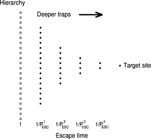
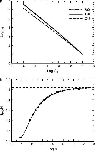
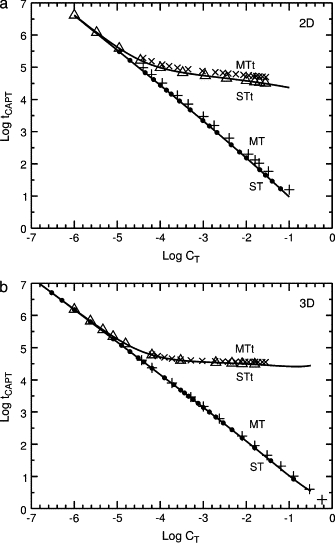
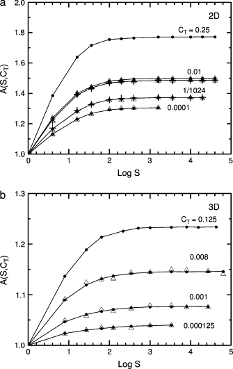
Reaction kinetics in a cell or cell membrane is modeled in terms of the first passage time for a random walker at a random initial position to reach an immobile target site in the presence of a hierarchy of nonreactive binding sites. Monte Carlo calculations are carried out for the triangular, square, and cubic lattices. The mean capture time is expressed as the product of three factors: the analytical expression of Montroll for the capture time in a system with a single target and no binding sites; an exact expression for the mean escape time from the set of lattice points; and a correction factor for the number of targets present. The correction factor, obtained from Monte Carlo calculations, is between one and two. Trapping may contribute significantly to noise in reaction rates. The statistical distribution of capture times is obtained from Monte Carlo calculations and shows a crossover from power-law to exponential behavior. The distribution is analyzed using probability generating functions; this analysis resolves the contributions of the different sources of randomness to the distribution of capture times. This analysis predicts the distribution function for a lattice with perfect mixing; deviations reflect imperfect mixing in an ordinary random walk.


Figures

Figure 1
Figure 1
A typical hierarchy of discrete traps and target, written as 16/8/4/2/T.
Figure 2
Figure 2
Capture times for a random walker in the presence of one target but no traps. (a) Log-log plot of the Montroll capture time tM as a function of the target concentration CT = 1/N for the two-dimensional case (triangular and square lattices) and the three-dimensional case (simple cubic lattice), from Eqs. 6 and 7 with coefficients given in the text. For the two-dimensional lattices, the theoretical results and the numerical results of Kozak are indistinguishable on the scale of this figure. (b) Scaled Monte Carlo capture times for the cubic lattice tM(3D)/N as a function of log N, and least-squares fit Eq. 7. Horizontal line, theoretical asymptotic limit imposed by Eq. 7.
Figure 3
Figure 3
Monte Carlo capture times for the standard trap hierarchy. Log-log plots of tCAPT as a function of the target concentration CT. (a) Triangular lattice. (b) Cubic lattice. Points: Monte Carlo results for single targets (ST, circles), multiple targets (MT, +), a single set of traps and target (STt, triangles), and multiple sets of traps and targets (MTt, ×). Lines: theoretical values, tCAPT = tM for single targets (ST) from Eqs. 6, 7 and tCAPT = tMtESC〉 for a single set of traps and targets (STt). In these examples the total concentration of traps and targets CTt = 31CT, so the total concentrations can be high; in the MTt series the maximum concentrations are CT = 0.02861, CTt = 0.8868 in panel a and CT = 0.02827, CTt = 0.8764 in panel b.
Figure 4
Figure 4
Dependence of the capture time on the number S of targets or sets of targets and traps for fixed target concentrations CT. Values of A(S, CT) are defined in Eq. 10. (a) Triangular and square lattices. (b) Cubic lattice. Note the changes in scale and CT. Circles and lines, targets but no traps; triangles, traps and targets. The standard hierarchy of traps is used, 16/8/4/2/T, PESC = 0.1. In panel a for CT = 0.01, the upper line is for the square lattice and the lower line is for the triangular lattice. Panel a also shows results for two alternative trap distributions on the triangular lattice, + for CT = 0.01, the continuous distribution of Eq. 11, and + for CT = 1/1024, the uniform discrete distribution 7/7/7/7/T. Runs were set up so that all concentrations and values of S were exact, although this limited the concentrations used. For example, when CT = 0.01, the first series of runs had only target sites at a fixed concentration and the system size was varied. There was one target in a 10 × 10 grid, four targets in a 20 × 20 grid, and so forth to 3600 targets in a 600 × 600 grid. The second series used the same target concentrations and grids but one set of 30 traps per target, so the total concentration was CTt = 0.31. For runs with targets and traps, 500 trap configurations were used, and 1000 tracers per trap configuration. For runs with traps alone, to get smooth curves 1000 trap configurations were used and 10,000 tracers per trap configuration.
Figure 5
Figure 5
Distribution of capture times from Monte Carlo calculations for the standard example, 16/8/4/2/T but with PESC = 0.2 so that all the curves can be shown conveniently on the same scale. Changes in noise levels within a curve are due to changes in bin width. Vertical lines at top, means. Notation in panels (ad): ST (red), single target but no traps; MT (blue), multiple targets but no traps; STt (green), single set of traps and target; MTt (purple), multiple sets of traps and targets. (a) Log fraction versus time for two dimensions, grid size 10 × 10 for the ST and STt curves, and 320 × 320 for the MT and MTt curves. (b) The same data versus log time to show the power-law region in the STt and MTt curves. (c) Log fraction versus time for three dimensions, grid size 5 × 5 × 5 for the ST and STt curves, and 50 × 50 × 50 for the MT and MTt curves. (d) The same data versus log time. The MT and MTt curves are for 1024 sets in two dimensions and 1000 in three dimensions. (e) The standard hierarchy 16/8/4/2/T (red) gives a power-law region but the uniform discrete distribution 7/7/7/7/T (green) and the continuous uniform distribution (blue) give more complicated curves. All three runs were on a 30 × 30 triangular lattice, and 5 million repetitions were used instead of the usual 0.5 million to separate the histograms more cleanly. (f) Increasing the number of levels in the hierarchy increases the size of the power-law region. The hierarchies used are 2/T, 4/2/T, 8/4/2/T, 16/8/4/2/T, 32/…/2/T, and 64/…/2/T with PESC = 0.1. For clarity the curves are shifted downward by 0, 1, 2, 3, 4, and 5 units, respectively. One target and set of traps was used on a triangular lattice. The system size was varied between 8 × 8 and 66 × 66 to keep the trap concentration as constant as possible, 0.02972 ± 0.00098; that is, an SD of 3.28% of the mean.
Figure 6
Figure 6
Probability distributions of capture times from the perfect-mixing approximation and Monte Carlo calculations. (a) Linear plot for the two-dimensional case. (b) Logarithmic plot for the two-dimensional case. Here gCAPT is a histogram of Monte Carlo capture times for a single target and no traps, and gCAPT_HIER (Eq. 19) combines gCAPT with gHIER to give the distribution for one set of traps and a target, assuming a fixed escape time from the traps. The final prediction, gCAPT_HIER_ESC (Eq. 21), also takes into account the distribution of escape times from traps. The Monte Carlo result for one set of traps and target is given by gMC. The distributions gCAPT_HIER and gCAPT_HIER_ESC are of significant magnitude well beyond 3000 time steps; the cumulative distribution functions for the Monte Carlo data at 3000 time steps are 0.568 in two dimensions and 0.654 in three. (c) Ratio of the Monte Carlo distribution to the calculated distribution log gMC/log gCAPT_HIER_ESC for the two-dimensional case, the three-dimensional case, and the complete graph. For the complete graph the ratio of the log coefficients was 0.9999 ± 0.0070 for 2500 time points. In all these calculations, to get smooth histograms large runs were used (104 trap configurations and 104 tracers per trap configuration).

References

    1. Saxton M.J. A biological interpretation of transient anomalous subdiffusion. I. Qualitative model. Biophys. J. 2007;92:1178–1191. - PMC - PubMed
    1. den Hollander F., Weiss G.H. Contemporary Problems in Statistical Physics. Society for Industrial and Applied Mathematics; Philadelphia, PA: 1994. Aspects of trapping in transport processes. 147–203.
    1. Kozak J.J. Chemical reactions and reaction efficiency in compartmentalized systems. Adv. Chem. Phys. 2000;115:245–406.
    1. Melo E., Martins J. Kinetics of bimolecular reactions in model bilayers and biological membranes. A critical review. Biophys. Chem. 2006;123:77–94. - PubMed
    1. Barzykin A.V., Seki K., Tachiya M. Kinetics of diffusion-assisted reactions in microheterogeneous systems. Adv. Colloid Interface Sci. 2001;89:47–140. - PubMed

Publication types

LinkOut - more resources