Landscape as a model: the importance of geometry

Abstract

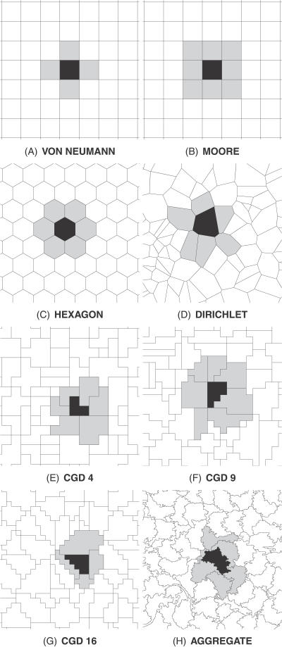
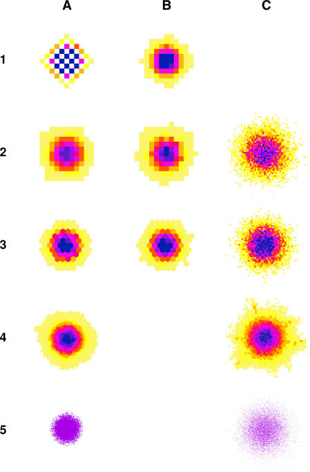
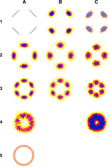
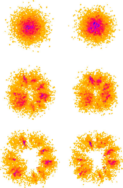
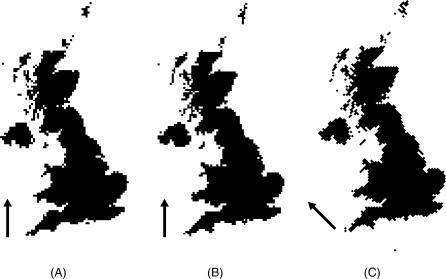
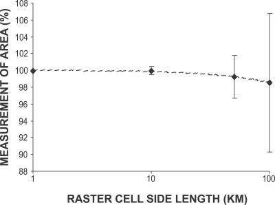
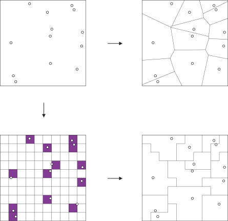
In all models, but especially in those used to predict uncertain processes (e.g., climate change and nonnative species establishment), it is important to identify and remove any sources of bias that may confound results. This is critical in models designed to help support decisionmaking. The geometry used to represent virtual landscapes in spatially explicit models is a potential source of bias. The majority of spatial models use regular square geometry, although regular hexagonal landscapes have also been used. However, there are other ways in which space can be represented in spatially explicit models. For the first time, we explicitly compare the range of alternative geometries available to the modeller, and present a mechanism by which uncertainty in the representation of landscapes can be incorporated. We test how geometry can affect cell-to-cell movement across homogeneous virtual landscapes and compare regular geometries with a suite of irregular mosaics. We show that regular geometries have the potential to systematically bias the direction and distance of movement, whereas even individual instances of landscapes with irregular geometry do not. We also examine how geometry can affect the gross representation of real-world landscapes, and again show that individual instances of regular geometries will always create qualitative and quantitative errors. These can be reduced by the use of multiple randomized instances, though this still creates scale-dependent biases. In contrast, virtual landscapes formed using irregular geometries can represent complex real-world landscapes without error. We found that the potential for bias caused by regular geometries can be effectively eliminated by subdividing virtual landscapes using irregular geometry. The use of irregular geometry appears to offer spatial modellers other potential advantages, which are as yet underdeveloped. We recommend their use in all spatially explicit models, but especially for predictive models that are used in decisionmaking.

Figure 1. Example Instances of Eight Virtual Landcapes

Example virtual landscape geometries (7 km × 7 km section). (A) von Neumann and (B) Moore neighbourhoods in a raster grid; (C) hexagonal; (D) Dirichlet tessellation; CGD tessellation with a mean of (E) four, (F) nine, and (G) 16 raster cells per km²; (H) land cover aggregate map. The neighbourhood (grey) of a focal cell (black) is highlighted in each virtual landscape.

Figure 2. Maximum Distance Accessible in 100 Steps

Maximum distance accessible in 100 cell-to-cell steps from the origin (star) in five virtual landscapes. The geometry of the regular grids is immediately apparent from the accessible regions of the von Neumann (yellow), Moore (red), and hexagonal (green) landscape models. Accessibility in all the irregular geometries was similar, and lay between that of the Dirichlet (circular blue line) and CGD4 (dashed circular blue line) virtual landscapes. London (shaded grey) is not accessible with some geometries, but is completely within reach of others.

Figure 3. Distribution of Step Lengths

The distribution of step lengths possible in five virtual landscapes. The von Neumann (orange, at 1.0) and hexagonal (green, at 1.074 km) landscapes only allow a single step length, whereas the Moore geometry allows two steps (red, at 1.0 and 1.41). A single instance of a Dirichlet landscape (blue, mean 1.095 km, gamma distributed with shape = 1.98, rate = 1.8 × 10⁴) allows a distribution of step lengths that vary from parcel to parcel but have a mean similar to the hexagonal geometry. Other irregular landscapes have step length distributed similarly (CGD4 shown, blue dashed line, mean 1.15 km).

Figure 4. Angular Variation in Accessibility

The minimum number of steps required to travel a range of distances was measured every 10° across a 90° angle in four virtual landscapes. The standard deviation increased linearly with increased distance (d) in the regular grids; von Neumann (dashed line) has trend 0.14d (R ² = 0.9995), Moore (dash dot) 0.09d (R ² = 0.9994), and hexagons (dash dot dot) 0.05d (R ² = 0.9952). Standard deviation in the Dirichlet virtual landscape (solid line) increased with trend 0.46 ln(d) (R ² = 0.968).

Figure 5. Population Distributions after Random Movement in Different Virtual Landscapes

A matrix showing population distributions after a number of random movement scenarios. Rows (from top to bottom): (1) von Neumann; (2) Moore; (3) hexagon; (4) Dirichlet; and (5) vector landscapes. Columns (from left to right): (A) random movement with t = 5 (time steps) and p = 1 (probability of movement in a time step); (B) random movement, t = 10, p = 0.5; and (C) random movement, t = 100, p = 1. Colours represent population density in each cell on a common scale, ranging from yellow (low density) through orange, red, and purple to blue (high density). In row 5, the vector points are only represented in one colour.

Figure 6. Population Distributions after Directed Random Movement in Different Virtual Landscapes

A matrix showing population distributions after a number of directed random movement scenarios. Rows (from top to bottom): (1) von Neumann; (2) Moore; (3) hexagon; (4) Dirichlet; and (5) vector landscapes. Columns (from left to right): (A) directed random movement, t = 50, p = 1, b = 0.0 (probability of backward movement); (B) directed random movement, t = 100, p = 0.5, b = 0.0; and (C) directed random movement, t = 50, p = 0.5, b = 0.1. Colours represent population density in each cell on a common scale, ranging from yellow (low density) through orange, red, and purple to blue (high density). In row (5), the vector points are only represented in one colour.

Figure 7. Random Movement in a Single Dirichlet Landscape

Population distributions in a Dirichlet landscape are shown after: (top) random movement with t = 100 (time steps), p = 1 (probability of movement in a time step); (centre) semi-directed movement with t = 50, p = 1, b = 0.1 (probability of choosing a neighbour closer to the origin); and (bottom) directed movement with t = 50, p = 1, b = 0. In the left column, individuals move into a neighbouring parcel with probability 1/(number of neighbours). In the right column, individuals move into a neighbouring parcel with probability proportional to the length of the shared boundary. There is no significant difference in the population distributions despite the difference in neighbour choice.

Figure 8. Qualitative Differences in Raster Representation of a Real Extent

Three alternative raster representations of the UK at 10 km resolution, formed against the BNG. In (A), the origin is at BNG (0,0) and the raster is aligned with the BNG. In (B), the origin has been shifted to BNG (−5000,−5000) but the orientation is unchanged. In (C), the origin is at BNG (0,0), but the raster has been rotated by 45°. The arrows refer to the orientation of the raster grid. Observe the variation in shape and size of the Orkney and Shetland isles (the two groups of islands north of the mainland).

Figure 9. Variation in the Area Measurement of a Real Extent

The area of the UK was measured from raster datasets at resolution 1, 10, 50, and 100 km, as a percentage of a vector polygon area (245,660 km²), and the mean calculated. The y-error bars denote coefficient of variation. The mean is always an underestimate, and worsens at lower resolutions.

Figure 10. Space and Direction from a Fixed Point in Multiple Irregular Landscapes

(A) A single Dirichlet landscape showing three fixed points (+). One (top left) occupies a cell inland, while another (top right) occupies a coastal cell that is restricted by the edge of the extent. The third (centre) is shown with the available directions for movement in that landscape instance. (B) A second random instance of a Dirichlet tessellation in the same extent. The three fixed points are highlighted, with their respective cells and directions of movement. (C) The sum of the observations of space and direction around the three points after only five Dirichlet landscapes. Light grey lines indicate the boundaries of cells in all five landscapes. The kernel associated with inland and coastal points is shown in shades of grey, with the lightest shade showing an area only associated with the point in one landscape instance and black being the area common to all five. Although clearly not circular, given enough iterations, all points approach a circular kernel of influence unless restricted by the extent. Available directions for movement across all five landscapes are shown from the third point, demonstrating that movement in any direction is equally possible.

Figure 11. Creation of a Coarse-Grain Dirichlet Landscape from a Raster

To create a Dirichlet landscape, starting points are chosen randomly (top left). The vector Dirichlet landscape (top right) is shown for comparison. Random starting points are translated into a raster grid (bottom left). All other raster squares are then assigned to the nearest coloured square (measured between centroids) and boundaries dissolved to produce the CGD landscape (bottom right).

References

-
- Lindenmayer DB, Fischer J, Hobbs R. The need for pluralism in landscape models: a reply to Dunn and Majer. Oikos. 2007;116:1419–1421.
- Wiens JA, Steneth NC, Van Horne B, Ims RA. Ecological mechanisms and landscape ecology. Oikos. 1993;66:369–380.
- Fuller RM, Smith GM, Sanderson JM, Hill JM, Thomson AG. The UK Land Cover Map 2000: construction of a parcel-based vector map from satellite images. Cartogr J. 2002;39:15–25.
- Kostova T, Carlsen T, Kercher J. Individual-based spatially-explicit model of an herbivore and its resource: the effect of habitat reduction and fragmentation. C R Biol. 2004;327:261–276. - PubMed
Publication types
MeSH terms
LinkOut - more resources
Full Text Sources