Topographic organization in and near human visual area V4

Abstract

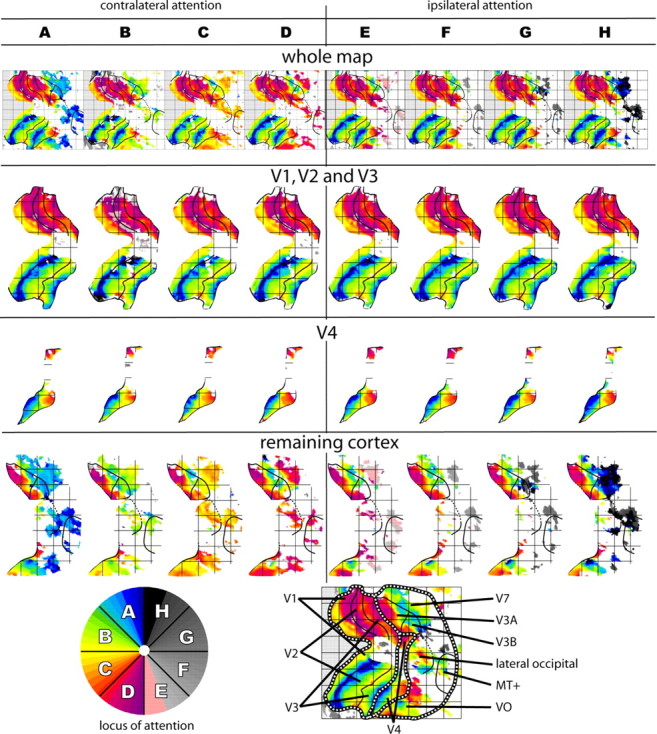
The existence and location of a human counterpart of macaque visual area V4 are disputed. To resolve this issue, we used functional magnetic resonance imaging to obtain topographic maps from human subjects, using visual stimuli and tasks designed to maximize accuracy of topographic maps of the fovea and parafovea and to measure the effects of attention on topographic maps. We identified multiple topographic transitions, each clearly visible in > or = 75% of the maps, that we interpret as boundaries of distinct cortical regions. We call two of these regions dorsal V4 and ventral V4 (together comprising human area V4) because they share several defining characteristics with the macaque regions V4d and V4v (which together comprise macaque area V4). Ventral V4 is adjacent to V3v, and dorsal V4 is adjacent to parafoveal V3d. Ventral V4 and dorsal V4 meet in the foveal confluence shared by V1, V2, and V3. Ventral V4 and dorsal V4 represent complementary regions of the visual field, because ventral V4 represents the upper field and a subregion of the lower field, whereas dorsal V4 represents lower-field locations that are not represented by ventral V4. Finally, attentional modulation of spatial tuning is similar across dorsal and ventral V4, but attention has a smaller effect in V3d and V3v and a larger effect in a neighboring lateral occipital region.

Figure 1.

Topography of human V1, V2, and V3 and macaque V4. Steps of transformations from the visual world and the cortical surface are shown as successive columns. The left column shows the visual field, with the upper field above and lower field below. Before visual information reaches the cortex, it is split into two halves (scissor icon) along the vertical meridian. The second column shows one visual hemifield using the same color legend as the actual fMRI maps (see remaining figures). In this and subsequent columns, the vertical cut is highlighted with circles. The third column shows how the visual hemifield is transformed further before reaching the cortical surface: the lower field is represented on top (i.e., dorsally), and the upper field is represented on the bottom (i.e., ventrally). The arrows link the same visual field locations before and after the transformation (purple-to-purple, blue-to-blue). The fourth column provides a rough illustration of how the visual field transformation might be distorted on the cortical surface. V1, Allman and Kaas (1974) named this type of transformation (a simple continuous map) a first-order transformation of the visual hemifield. V2, This transformation resembles V1 in most respects but includes an additional cut that does not follow the vertical meridian (additional scissors icon and stars). The off-vertical cut splits apart the dorsal and ventral portions (top and bottom, two rightmost panels). Allman and Kaas (1974) named this type of split transformation second order. The V2 and V1 transformations also differ in that V2 is not mirror reversed (upper-to-lower angles run roughly counterclockwise in the V2 panel but in the opposite direction in V1). Visual field coverage in V2d and V2v are complementary (i.e., each region represents part of the hemifield that the other does not). V3, The transformation resembles that of V2, except that it is mirror reversed. V4, The macaque V4 visual field transformation resembles that of V2, except that the off-vertical visual field cut is not always along the horizontal. In some individual macaques, it runs through the lower field, such that both V4d and V4v include some lower-field representation. However, visual field coverage in V4d and V4v (like that in V2d and V2v) are still complementary. V4 (like V2) is a non-mirror-reversed second-order transformation. The top black and white V4 panels are adapted from Figure 22 of Gattass et al. (1988).

Figure 2.

Stimuli and tasks. A, Foveal angle-mapping stimuli. A wedge, 90° in angular width and 5.1° in radial eccentricity, rotated around a fixation point in continuous motion. The texture within the wedge was a high (100%)-contrast, black-and-white radial checkerboard, scaled exponentially. The texture inside the circle swept out by the wedge (but outside the wedge itself) was the same checkerboard at low (2%) contrast. The screen outside this circle was isoluminant gray. Both the high- and the low-contrast textures rotated around the fixation point at the same speed as the wedge (one period was 36 s). B, Foveal eccentricity-mapping stimuli. A ring (the thickness of which was scaled logarithmically with distance from fixation) expanded or contracted around the fixation point in discrete jumps. The maximal eccentricity subtended by the ring was 5.1 radial degrees. At all positions, the ring was as wide as two checks. C, Peripheral angle-mapping stimuli. The m-sequence controlling wedge presentation was 255 frames long; onset time is indicated above each image. The figure suggests static images, but the phase of each grating was varied systematically to produce a dynamic animation. D, Peripheral eccentricity-mapping stimuli. The same m-sequence as in C controlled the presentation of four individual rings, of thickness scaled with distance from fixation. The underlying grating texture and timing parameters were the same as those used for the wedges. E, Attention task. The mapping experiment was repeated a multiple of eight times (wedge, shown here) or four times (ring). Each time, the subject fixated a central cross and covertly attended the texture in a different wedge or ring. F, Control task. Subjects reported subtle changes in luminance in a small (0.3°) circle around the fixation cross. The stimuli were identical to those used in the attention task.

Figure 3.

Transitions used as boundary criteria. Each transition indicated by a letter in the figure is described in detail in the text and is clearly visible in at least 75% of the 16 hemispheres with 2 × 2 × 2 mm voxel data. The terms “working boundary” and “peripheral observed boundary” are defined in the text. A, V1/V2; B, V2/V3; C, V3d/V3A; D, V3d/V3B; E, V3d/dorsal V4; F, dorsal V4/V3B; G, working V3B/V3A boundary; H, anterior boundary of V3A; I, anterior boundary of V3B; J, V3v/ventral V4; K, peripheral observed boundary of V1; L, peripheral observed boundary of V2; M, peripheral observed boundary of V3; N, peripheral observed boundary of V3A; O, peripheral observed boundary of upper-field ventral V4; P, peripheral observed boundary of lower-field ventral V4; Q, posterior/lateral boundary of lower-field ventral V4; R, lateral boundary of upper-field ventral V4; S, dorsal V4/lateral occipital; T, peripheral observed boundary of dorsal V4; U, inferior boundary of lateral occipital; V, peripheral observed boundary of lateral occipital.

Figure 4.

Right-hemisphere (RH) foveal/parafoveal maps. Maps from subjects 1–4 (S1–S4) are shown. (For the left-hemisphere maps from the same subjects and for maps from both hemispheres of subjects 5–8, see supplemental figures, available at www.jneurosci.org as supplemental material.) A, Eccentricity maps. Solid lines indicate boundary criteria as in Figure 3. Points where the SE on the phase exceeded 3 s are thresholded out of the map (white). B, Angle maps, formatted as in A. In these and all other angle maps in this study, the upper vertical meridian is shown as dark blue, the horizontal meridian is shown as yellow, and the lower vertical meridian is shown as purple. Green and orange correspond to intermediate upper- and lower-field angles, respectively. C, Top row, inferodorsal view of the inflated hemisphere, selected to maximize visibility of cortex both dorsal and ventral to the foveal confluence; bottom row, posteromedial view of the inflated hemisphere, selected to maximize visibility of V1.

Figure 5.

Visual field coverage in the central 5° of V1, V2, V3, and V4. Each polar plot shows the portion of the central 5° observed within one ROI. Peak eccentricity and angle tuning at each point on the virtual cortical surface appear as the radial distance and angular value of each point on the plot. The number of 2 × 2 × 2 mm voxels that intersect each ROI is shown at the top right of each plot, indicating how the voxel data correspond to the displayed surface data. Red points are from the left hemisphere, and blue points are from the right hemisphere. The V1, V2, and V3 data represent the entire stimulated hemifield; what patchiness exists in these plots presumably reflects measurement artifacts such as those reported previously (Dougherty et al., 2003). The V4 data represent the entire stimulated hemifield (see also Fig. 6). The lateral occipital (lat. occ.) data represent most angles in most hemispheres, but there is a consistent gap in the middle stimulated eccentricities (see Results). The V3A and V3B data represent most angles in most subjects, but there is a consistent gap in the central visual field (see Results).

Figure 6.

Complementary visual field coverage in dorsal and ventral V4. A, The V4 data from Figure 5 are divided into ventral V4 (top, purple), dorsal V4 (middle, green), and V4 as a whole (bottom, overlapping purple and green). Across subjects and hemispheres, the ventral V4 data consistently do not cover the parafoveal lower visual field, but the dorsal V4 data do, and area V4 data as a whole cover the entire stimulated visual field. B, Each numeral gives the number of hemispheres (of 12) in which the estimated spatial tuning of at least two surface vertices in ventral V4 (left) or dorsal V4 (right) was within the corresponding sector. The sectors are shown to scale; each is 1° of eccentricity by 30° of polar angle. C, The same information as in B is represented graphically. Two key observations are apparent. First, visual field coverage in dorsal V4 is complementary to visual field coverage in ventral V4 (compare similar observation in macaque V4 in Fig. 1). Second, the visual field cut that splits the dorsal and ventral portions is typically not along the horizontal meridian, as is the case in the more familiar areas V2 and V3. Instead, the visual field cut tends to occur at intermediate lower-field angles (compare macaque V4 in Fig. 1).

Figure 7.

Modulation of spatial tuning by attention: map examples. Columns A–H show angular mapping data acquired during attention to a single contralateral wedge. The scale at the bottom left indicates the attended wedge for each panel. Top row, Each map represents one-eighth of the data acquired from subject 1 right hemisphere. The more that attention shifts the spatial tuning estimates, the more the colors change across columns. To aid visualization, the maps in the top row have been divided into three parts: V1/V2/V3 (second row), where attentional modulations are negligible and the colors barely change; V4 (third row), where attentional modulations are moderate and the colors change slightly; the remainder of cortex on the map (bottom row), including regions where attentional modulations are dramatic and the colors change vividly.

Figure 8.

Modulation of spatial tuning by attention: ROI analysis. ROIs were defined in all hemispheres in which both foveal/parafoveal data (for dorsal V4 ROI assignment) and attentional data (for attention analysis) were available. The ROIs themselves were defined by the foveal/parafoveal data, and the data analyzed within the ROIs are the attentional data. The top row shows upper-field ROIs; the bottom row shows lower-field ROIs. Modulation of spatial tuning by attention is quantified as S_match. This index increases as spatial tuning shifts toward the attended wedge, and it is not artificially inflated by noise. An unmodulated ROI would have an S_match of 1; larger values represent greater modulation toward attended wedges (upper limit 8). Error bars give the SE, calculated for each ROI by jackknifing. S_match in upper-field ventral V4, lower-field ventral V4, and lower-field dorsal V4 are not significantly different from one another but are significantly different from S_match in both upper- and lower-field portions of the neighboring regions V3 and lateral occipital (lat-occ). LH, Left hemisphere; RH, right hemisphere.

Figure 9.

Macaque V4 and human V4. Data are formatted as in Figure 1. To aid in comparison, the top row is repeated from the bottom row of Figure 1 (macaque V4); the plots represent neurophysiological responses to stimuli located at ≤30°. The bottom two rows depict the organization observed in two individual human subjects; these plots represent fMRI spatial tuning estimates to stimuli located at ≤5°. The figure as a whole illustrates that macaque V4 and human V4 share remarkably similar topographic organizations.

Figure 10.

Our V4 parcellation versus alternative parcellations (hV4+LO1 and V4v/V4d-topo+V8). A, Right-hemisphere maps from our subject 2. This hemisphere is very similar to that in the first exemplar hemisphere from the LO1 study [the right hemisphere of subject 8 in Fig. 1 of Larsson and Heeger (2006) (LH 2006)]. In both, an elongated patch of upper-field angles appears within lateral occipital, roughly parallel to the anterior boundary of parafoveal V3d. This patch is the defining feature of the putative LO1 anterior boundary (dark blue arrow, as in the dark blue top vertical meridian; compare our anterior dorsal V4 boundary, marked with a yellow arrow as in the yellow horizontal meridian). B, Right-hemisphere maps from our subject 1. As in A, the ventral V4 data do not include parafoveal-stimulated eccentricities at lower-field angles. However, in this hemisphere, the lateral occipital topographic patterns do not include the defining feature of the LO1/LO2 boundary, described above. Instead, multiple reversing upper- and lower-field stripes run roughly at right angles to the isoangle contours in dorsal V4 and to the parafoveal V3d boundary. C, The relationship between our V4 and V4v/V4d-topo+V8 is illustrated as a schematic adapted from that in Tootell and Hadjikhani (2001) (TH 2001). The V4v/V4d-topo scheme predicted that in the future, a V4d parallel would be found within V4d-topo (lavender); our dorsal V4 (yellow overlay) fulfills that prediction. D, A series of tests demonstrates that our V4 scheme (HKG) accounts better for the available data than hV4+LO1 or V4v/V4d-topo+V8. ①, Point 1 was central to Tootell and Hadjikhani (2001). ②, The hV4+LO1 scheme requires hV4 to be a complete hemifield. Problematically, the LO1/LO2 scheme describes hV4 as a hemifield, but the hV4 visual field coverage plots (Larsson and Heeger, 2006) are closer to quadrant V3v. ③, Uniquely human features in visual cortex are rare enough to be perceived as exceptional (Preuss 2004), so claims of human uniqueness require compelling data (see Discussion).

Figure 11.

Our V4 parcellation in a chronological context. The locations of various regions described in the literature are shown. Because the ventral map literature has been particularly controversial, the figure focuses on a ventral view. The figure does not include the converging lines of evidence that support our scheme over hV4+LO1 and V4v/V4d-topo+V8; for this material, see Figure 10 and the Discussion. The panels show a single map segmented according to boundaries used in several studies that focused on different aspects of the data. We attempt to portray each set of boundaries objectively, but the figures in the original studies may better reflect the authors' intended claims. The map itself is from our parafoveal/peripheral across-attention dataset (subject 1 LH), which provides good coverage of the peripheral region where several boundary schemes overlap. The central small white disk in the angle color legend is a reminder that the central ±1° was unstimulated in the parafoveal/peripheral angle experiments (see Materials and Methods). The eccentricity color legend is scaled to account for the center-of-mass bias inherent in the analysis of the eccentricity m-sequence data (see Materials and Methods) and uses different colors to avoid confusion with the foveal/parafoveal maps in previous figures. U, Upper visual field; L, lower visual vield; UL, both upper and lower visual field; CaS, calcarine sulcus; POS, parieto-occipital sulcus; CoS, collateral sulcus; FuG, fusiform gyrus. A, Field-sign-defined V4v (no dorsal component defined). B, Meridian-defined V4v (no dorsal component defined). C, V4v, as in B, and V8. D, hV4 (no dorsal component defined), VO-1, and VO-2. E, V4 (equivalent to hV4; no dorsal component defined), VMO, and VOF. F, Ventral V4 (paired with dorsal V4). Ventral V4 overlaps with field-sign-defined V4v, with meridian-defined V4v plus additional cortex, with a small part of V8, with hV4 plus additional cortex (as shown here, plus the extension of the upper field into the foveal confluence visible in the foveal/parafoveal data from Fig. 4), and with part of VMO. Ventral V4 does not overlap with the majority of V8, with VO-1, or VO-2 (given some variability at farthest-peripheral upper-field ventral V4), or with VOF.

References

1. Allman JM, Kaas JH. The organization of the second visual area (VII) in the owl monkey: a second order transformation of the visual hemifield. Brain Res. 1974;76:247–265. - PubMed
1. Boussaoud D, Ungerleider LG, Desimone R. Pathways for motion analysis: cortical connections of the medial superior temporal and fundus of the superior temporal visual areas in the macaque. J Comp Neurol. 1990;296:462–495. - PubMed
1. Brainard DH. The psychophysics toolbox. Spat Vis. 1997;10:433–436. - PubMed
1. Brefczynski JA, DeYoe EA. A physiological correlate of the “spotlight” of visual attention. Nat Neurosci. 1999;2:370–374. - PubMed
1. Brewer AA, Press WA, Logothetis NK, Wandell BA. Visual areas in macaque cortex measured using functional magnetic resonance imaging. J Neurosci. 2002;22:10416–10436. - PMC - PubMed
LinkOut - more resources