Modeling the bicoid gradient: diffusion and reversible nuclear trapping of a stable protein

Abstract

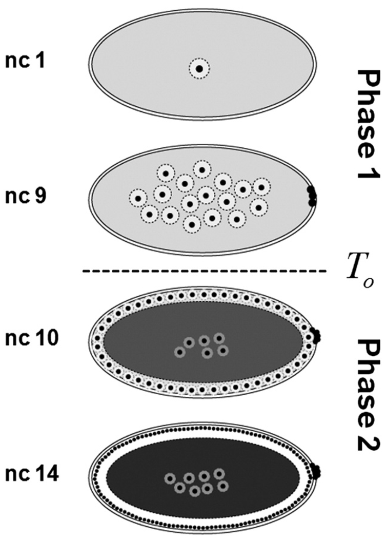
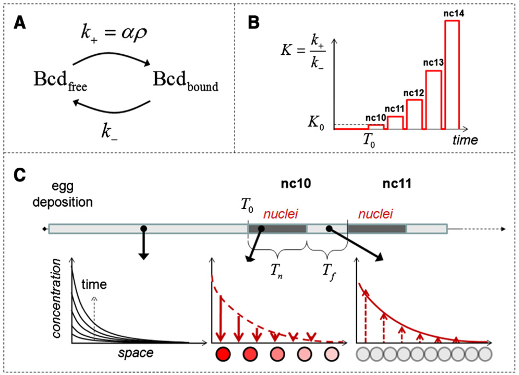
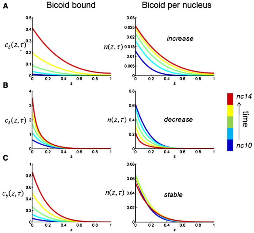
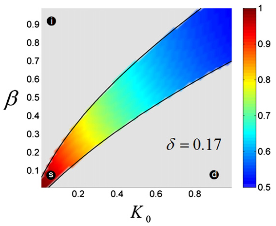
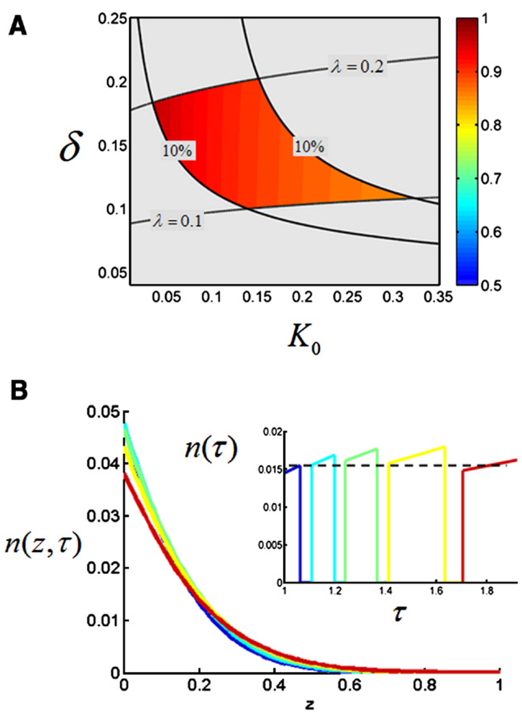
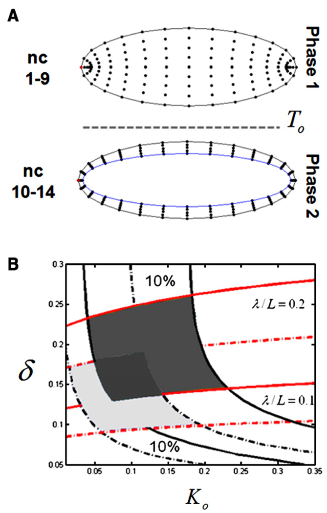
The Bicoid gradient in the Drosophila embryo provided the first example of a morphogen gradient studied at the molecular level. The exponential shape of the Bicoid gradient had always been interpreted within the framework of the localized production, diffusion, and degradation model. We propose an alternative mechanism, which assumes no Bicoid degradation. The medium where the Bicoid gradient is formed and interpreted is very dynamic. Most notably, the number of nuclei changes over three orders of magnitude from fertilization, when Bicoid synthesis is initiated, to nuclear cycle 14 when most of the measurements were taken. We demonstrate that a model based on Bicoid diffusion and nucleocytoplasmic shuttling in the presence of the growing number of nuclei can account for most of the properties of the Bicoid concentration profile. Consistent with experimental observations, the Bicoid gradient in our model is established before nuclei migrate to the periphery of the embryo and remains stable during subsequent nuclear divisions.

Fig. 1

Summary of changes in the number and distribution of nuclei in the syncytial embryo. Following egg deposition, nuclei divide thirteen times in a common cytoplasm. This process stage can be split into two temporal phases. During phase one (nuclear cycles 1 to 9), nuclei are distributed in the bulk of the embryo and surrounded by cytoplasmic islands. At nuclear cycle 10 nuclei move to the outer plasma membrane and a clear rim of cytoplasm appears at the cortex of the embryo. During phase two (nuclear cycles 10 to 14), nuclei are distributed under the plasma membrane. At this stage, yolk occupies the center of the embryo and appears to be impermeable to Bicoid.

Fig. 2

Model of Bicoid diffusion and reversible trapping by nuclei, see text for details. (A) Bicoid exists in two states: freely diffusing and immobile/nuclear. The transitions between the two states are described by first-order processes. The forward nuclear trapping rate constant is proportional to the nuclear density. (B) The time-dependent nuclear density in the syncytial embryo is translated into the time-dependent equilibrium constant for the nucleocytoplasmic shuttling of Bicoid (see text for details). nc10, nc11, etc. denote the nuclear cycles 10, 11, etc. (C) Schematic representation of the dynamics of the Bicoid gradient. From t = 0 to t = T₀, Bicoid diffusion is essentially unaffected by nuclei. This “free-diffusion” phase (bottom left panel; curves represent diffusive spread of Bicoid from the constant source the boundary) is followed by the phase with much greater value of the nucleocytoplasmic shuttling equilibrium constant. Each of the five nuclear cycles during this phase is in turn composed of two stages, with and without the nuclei. T_n,i and T_f,i denotes the durations of the nuclear and free periods, respectively. The gradient of nuclear Bicoid is formed at the beginning of each nuclear cycle (bottom middle panel). When nuclei dissolve Bicoid is again freely diffusing (bottom right panel).

Fig. 3

Computational analysis of the simplified model in which the durations of the nuclear and free portions of the nuclear cycles are constant. The local dimensionless concentration of Bicoid molecules in the bound state, c_b (z), is always increasing (left), however the local concentration of the Bicoid molecules per nucleus (n(z), right) can increase, decrease, and remain quasi-invariant with time. Examples A–C correspond to the following values of model parameters: A − δ = 0.17, K₀ = 0.01, β = 1, γ = 1; B − δ = 0.17, K₀ = 0.9, β = 0.2, γ = 1; C − δ = 0.17, K₀ = 0.05, β = 0.2, γ = 1. The plot shows the results of numerical solution of the dimensionless problem; see Materials and methods for the details of nondimensionalization and numerical methods.

Fig. 4

Stable gradients in the simplified model. The shaded region in the (β, K₀) plane corresponds to nuclear gradients that are at least 10% accurate over the five last nuclear cycles; see Materials and methods for the description of the accuracy criterion. The region has been computed for γ = 1 and δ = 0.17. The gradients above this region are steadily increasing as a function of nuclear density, while those below this region are steadily decreasing. The black circles correspond to the increasing (i), decreasing (d), and stable (s) gradients shown in Fig. 3. The color shading of the region shows the ratio of the widths (second moments) of the gradients, n(z, t), with and without the nuclei; see Materials and methods for details.

Fig. 5

Model-based analysis of quantitative measurements of the Bicoid gradient. (A) Specifying the times of nuclear divisions leaves δ and K₀ as the only free parameters in the model. Their values are constrained to the shaded region by the experimental measurements of the shape and the accuracy of the Bicoid gradients. The shaded region is bounded by four sets of curves. The gradients above the upper curve are too shallow, while the ones below the bottom curve are too sharp. The sharpness of the gradient is determined by fitting it to an exponential profile; λ is the parameter of the fit. The bounds for the allowable range of the values of λ is provided by the experimentally available information about the distribution function of gradient decay lengths (Gregor et al., 2005). At the same time, only the gradients between the vertical lines satisfy the criterion of 10% accuracy over the five last nuclear divisions. (B) Dynamics of the gradient of nuclear Bicoid, n(z, r), computed for δ and K₀ inside the data consistency region. The inset shows the time course of the nuclear levels of Bicoid at z = 0.2, computed for K₀ = 0.15, δ = 0.15.

Fig. 6

Analysis of the three-dimensional model. (A) Finite difference grids used to solve the problem in the prolate spheroidal coordinate system (see text for details). (B) Comparison of the regions of the parameter space consistent with the experimentally derived quantitative properties of the Bicoid gradient: light gray—one-dimensional model, dark gray—three-dimensional model.

References

-
- Abramowitz M, Stegun IA. Handbook of Mathematical Tables with Formulas, Graphs, and Mathematical Tables. Washington: Dover Pubns; 1964.
- Bressloff PC, Earnshaw BA. Diffusion-trapping model of receptor trafficking in dendrites. Phys. Rev. 2007:E 75. - PubMed
- Casanova J, Struhl G. The torso receptor localizes as well as transduces the spatial signal specifying terminal body pattern in Drosophila. Nature. 1993;362:152–155. - PubMed
- Chen Y, Struhl G. Dual roles for patched in sequestering and transducing hedgehog. Cell. 1996;87:553–563. - PubMed
MeSH terms
Substances
Grants and funding
LinkOut - more resources
Full Text Sources
Molecular Biology Databases