Experimental design for efficient identification of gene regulatory networks using sparse Bayesian models

Abstract

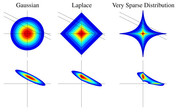
Background: Identifying large gene regulatory networks is an important task, while the acquisition of data through perturbation experiments (e.g., gene switches, RNAi, heterozygotes) is expensive. It is thus desirable to use an identification method that effectively incorporates available prior knowledge - such as sparse connectivity - and that allows to design experiments such that maximal information is gained from each one.

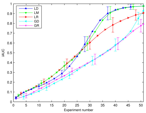
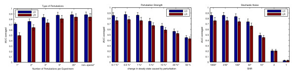
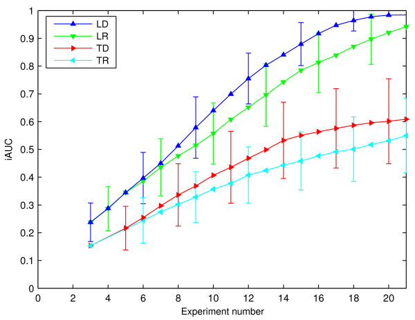
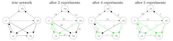
Results: Our main contributions are twofold: a method for consistent inference of network structure is provided, incorporating prior knowledge about sparse connectivity. The algorithm is time efficient and robust to violations of model assumptions. Moreover, we show how to use it for optimal experimental design, reducing the number of required experiments substantially. We employ sparse linear models, and show how to perform full Bayesian inference for these. We not only estimate a single maximum likelihood network, but compute a posterior distribution over networks, using a novel variant of the expectation propagation method. The representation of uncertainty enables us to do effective experimental design in a standard statistical setting: experiments are selected such that the experiments are maximally informative.

Conclusion: Few methods have addressed the design issue so far. Compared to the most well-known one, our method is more transparent, and is shown to perform qualitatively superior. In the former, hard and unrealistic constraints have to be placed on the network structure for mere computational tractability, while such are not required in our method. We demonstrate reconstruction and optimal experimental design capabilities on tasks generated from realistic non-linear network simulators. The methods described in the paper are available as a Matlab package athttp://www.kyb.tuebingen.mpg.de/sparselinearmodel.

Figure 1

The Choice of Model. Three prior distribution candidates over network matrix coefficients: Gaussian, Laplace, and "very sparse" distribution (P(a_ij) ∝ exp(- τ|a_ij|^0.4)). We show contour plots of density functions over two entries, coloured areas contain the same probability mass for each of the distributions. Upper row: prior distributions (unit variance), and likelihood for single measurement (linear constraint with Gaussian uncertainty). Lower row: corresponding posterior distributions. The Gaussian is spherically distributed, the others shift probability mass towards the axes, giving more mass to sparse tuples (≥ 1 entry close to 0). This effect is clearly visible in the posterior distributions. For the Gaussian prior, the area close to the axes has rather low mass. The Laplace-posterior is skewed: more mass is concentrated close to the vertical axis. Both posteriors are log-concave (and unimodal). The "very sparse"-posterior is shrunk towards the axes more strongly, sparsity is enforced stronger than for the Laplace prior. But it is bimodal, giving two different interpretations for the single observation. This multimodality increases exponentially with the number of dimensions, rendering accurate inference very difficult. The Laplace prior therefore is a good compromise between computational tractability and suitability of the model.

Figure 2

An Example Network. Small-world network of N = 50 nodes. Arrowless edges are bi-directional. "Gene names" are randomly drawn. Some nodes have rather high in-degree, characteristic of real biological networks, e.g. [18].

Figure 3

Reconstruction Performance for Different Methods. Reconstruction curves for experiments (gene expression changes of 1%, SNR 100, r = 3 non-zeros per u). LD: Laplace prior, experimental design. LR: Laplace prior, random experiments. GD: Gaussian prior, experimental design. GR: Gaussian prior, random experiments. LM: Laplace prior, mixed selections (first 20 random, then designed). Error bars show one standard deviation over runs. All visually discernible differences in mean curves of different methods are significant under the t-test at level 1%.

Figure 4

Reconstruction Performance for Different Experimental Conditions. Comparison between LD (Laplace, design) and LR (Laplace, random experiments) under different conditions. Score is average iAUC after 25, ..., 50 experiments. (Left): Number r of non-zero u coefficients in each disturbance varied, keeping ||u|| constant. (Middle): Norm ||u|| of disturbances varied, while keeping r = 3 and low noise level. (Right): Stochastic noise in the data (1) varied, for constant ||u||, r = 3. Settings marked with *: LD is significantly superior to LR, according to t-test at level 1%.

Figure 5

Reconstruction Performance Compared to Tegnér et. al. Network recovery performance, comparing our method (Laplace, design) with [3]. Networks of size N = 20, r = 1 non-zeros in u, perturbation size 1%, SNR 100. Three initial random experiments, to reduce memory requirements in [3] method. TD: [3], experimental design. TR: [3], random experiments. LD: Our method, Laplace prior, experimental design. LR: Our method, Laplace prior, random experiments.

Figure 6

Reconstruction of Drosophila segment polarity network. The left figure shows the effective single cell model with five genes of the Drosophila segment polarity network [24]. Lines with circles denote inhibitory, arrows activating influence, functionally weak links are dashed. The figures on the right show the ranks that our algorithm assigns to each of the edges after n experiments (n = 2, 4, 5). There are 6 rel. strong edges with $\tilde{A}$_ij ≠ 0 in the network, and we assume that an edge is correctly identified if its rank is amoung the top 6. These edges are coloured green.

References

1. Yeung MKS, Tegnér J, Collins JJ. Reverse engineering gene networks using singular value decomposition and robust regression. PNAS. 2002;99:6163–6168. doi: 10.1073/pnas.092576199. - DOI - PMC - PubMed
1. Kholodenko BN, Kiyatkin A, Bruggeman FJ, Sontag E, Westerhoff HV, Hoek JB. Untangling the wires: A strategy to trace functional interactions in signaling and gene networks. PNAS. 2002;99:12841–12846. doi: 10.1073/pnas.192442699. - DOI - PMC - PubMed
1. Tegnér J, Yeung MKS, Hasty J, Collins JJ. Reverse engineering gene networks: Integrating genetic perturbations with dynamical modeling. PNAS. 2003;100:5944–5949. doi: 10.1073/pnas.0933416100. - DOI - PMC - PubMed
1. Sontag E, Kiyatkin A, Kholodenko BN. Inferring dynamic architecture of cellular networks using time series of gene expression, protein and metabolite data. Bioinformatics. 2004;20:1877–1886. doi: 10.1093/bioinformatics/bth173. - DOI - PubMed
1. Schmidt H, Cho KH, Jacobsen E. Identification of Small Scale Biochemical Networks based on General Type System Perturbations. FEBS. 2005;272:2141–2151. doi: 10.1111/j.1742-4658.2005.04605.x. - DOI - PubMed
LinkOut - more resources