Review on solving the forward problem in EEG source analysis

Abstract

Background: The aim of electroencephalogram (EEG) source localization is to find the brain areas responsible for EEG waves of interest. It consists of solving forward and inverse problems. The forward problem is solved by starting from a given electrical source and calculating the potentials at the electrodes. These evaluations are necessary to solve the inverse problem which is defined as finding brain sources which are responsible for the measured potentials at the EEG electrodes.

Methods: While other reviews give an extensive summary of the both forward and inverse problem, this review article focuses on different aspects of solving the forward problem and it is intended for newcomers in this research field.

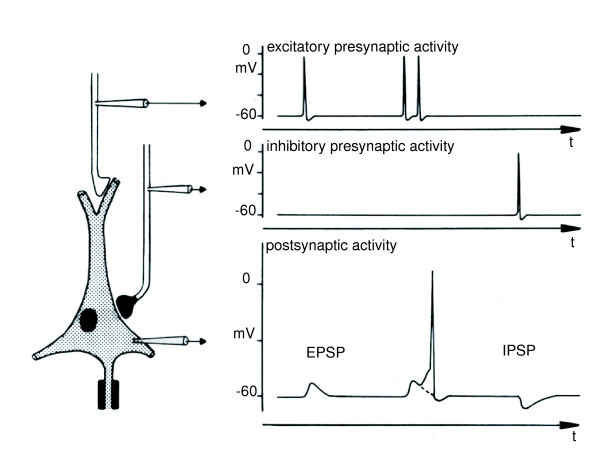
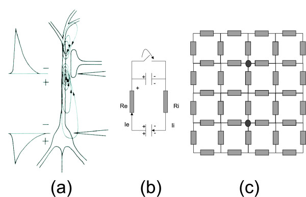
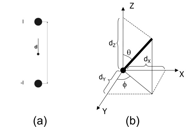
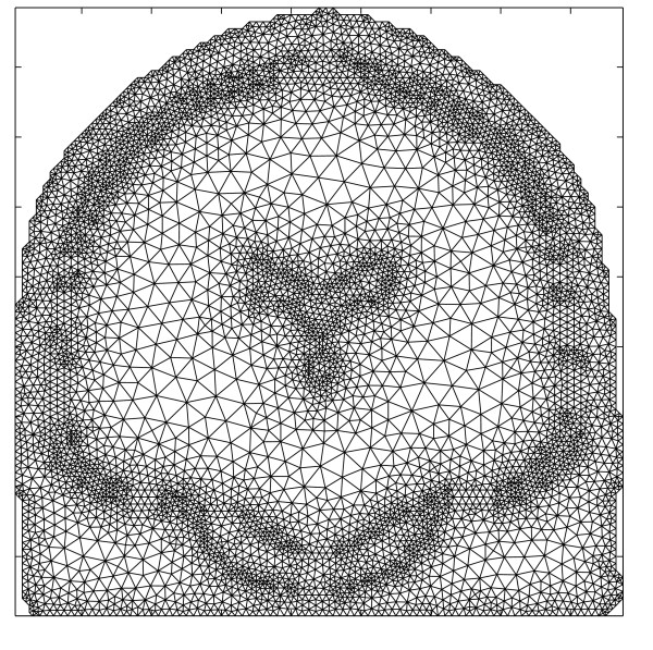
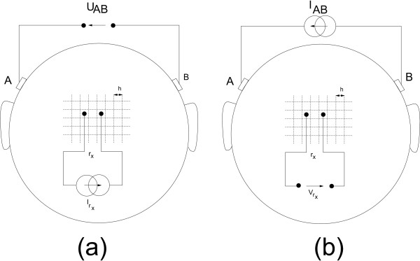
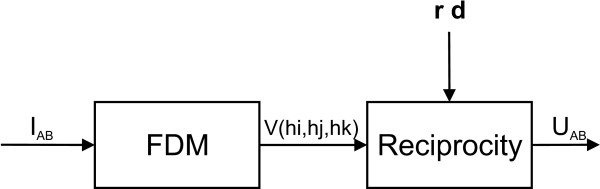
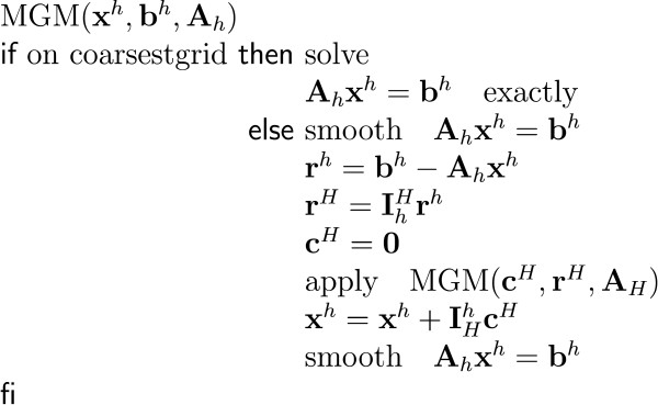
Results: It starts with focusing on the generators of the EEG: the post-synaptic potentials in the apical dendrites of pyramidal neurons. These cells generate an extracellular current which can be modeled by Poisson's differential equation, and Neumann and Dirichlet boundary conditions. The compartments in which these currents flow can be anisotropic (e.g. skull and white matter). In a three-shell spherical head model an analytical expression exists to solve the forward problem. During the last two decades researchers have tried to solve Poisson's equation in a realistically shaped head model obtained from 3D medical images, which requires numerical methods. The following methods are compared with each other: the boundary element method (BEM), the finite element method (FEM) and the finite difference method (FDM). In the last two methods anisotropic conducting compartments can conveniently be introduced. Then the focus will be set on the use of reciprocity in EEG source localization. It is introduced to speed up the forward calculations which are here performed for each electrode position rather than for each dipole position. Solving Poisson's equation utilizing FEM and FDM corresponds to solving a large sparse linear system. Iterative methods are required to solve these sparse linear systems. The following iterative methods are discussed: successive over-relaxation, conjugate gradients method and algebraic multigrid method.

Conclusion: Solving the forward problem has been well documented in the past decades. In the past simplified spherical head models are used, whereas nowadays a combination of imaging modalities are used to accurately describe the geometry of the head model. Efforts have been done on realistically describing the shape of the head model, as well as the heterogenity of the tissue types and realistically determining the conductivity. However, the determination and validation of the in vivo conductivity values is still an important topic in this field. In addition, more studies have to be done on the influence of all the parameters of the head model and of the numerical techniques on the solution of the forward problem.

Figure 1

Excitatory and inhibitory post synaptic potentials. An illustration of the action potentials and post synaptic potentials measured at different locations at the neuron. On the left a neuron is displayed and three probes are drawn at the location where the potential is measured. The above picture on the right shows the incoming exitatory action potentials measured at the probe at the top, at the probe in the middle the incoming inhibitory action potential is measured and shown. The neuron processes the incoming potentials: the excitatory action potentials are transformed into excitatory post synaptic potentials, the inhibitory action potentials are transformed into inhibitory post synaptic potentials. When two excitatory post synaptic potentials occur in a small time frame, the neuron fires. This is shown at the bottom figure. The dotted line shows the EPSP, in case there was no second excitatory action potential following. From [2].

Figure 2

equivalent circuit for a neuron. An excitatory post synaptic potential, an simplified equivalent circuit for a neuron, and a resistive network for the extracellular environment. A neuron with an excitatory synapse at the apical dendrite is presented in (a). From [2]. A simplified equivalent circuit is depicted in (b). The extracellular environment can be represented with a resistive network as illustrated in (c).

Figure 3

The current density and equipotential lines in the vicinity of a dipole. The current density and equipotential lines in the vicinity of a current source and current sink is depicted. Equipotential lines are also given. Boxes are illustrated which represent the volumes G.

Figure 4

Anisotropic conductivity of the brain tissues. The anisotropic properties of the conductivity of skull and white matter tissues. The anisotropic properties of the conductivity of skull and white matter tissues. (a) The skull consists of 3 layers: a spongiform layer between two hard layers. The conductivity tangentially to the skull surface is 10 times larger than the radial conductivity. (b) White matter consist of axons, grouped in bundles. The conductivity along the nerve bundle is 9 times larger than perpendicular to the nerve bundle.

Figure 5

The boundary between two compartments. The boundary between two compartments. The boundary between two compartments, with conductivity σ₁ and σ₂. The normal vector e_n to the interface is also shown.

Figure 6

The dipole parameters. (a) The dipole parameters for a given current source and current sink configuration. (b) The dipole as a vector consisting of 6 parameters. 3 parameters are needed for the location of the dipole. 3 other parameters are needed for the vector components of the dipole. These vector components can also be transformed into spherical components: an azimuth, elevation and magnitude of the dipole.

Figure 7

The equipotential lines of a dipole. The equipotential lines of a dipole oriented along the z-axis. The numbers correspond to the level of intensity of the potential field generated of the dipole. The zero line divides the dipole field into two parts: a positive one and a negative one.

Figure 8

The three-shell concentric spherical head model. The dipole is located on the z-axis and the potential is measured at scalp point P located in the xz-plane.

Figure 9

Example mesh of the human head used in BEM. Triangulated surfaces of the brain, skull and scalp compartment used in BEM. The surfaces indicate the different interfaces of the human head: air-scalp, scalp-skull and skull-brain.

Figure 10

Example mesh in 2D used in FEM. A digitization of the 2D coronal slice of the head. The 2D elements are the triangles.

Figure 11

The computation stencil used in FDM. A typical node P in an FDM grid with its neighbours Q_i (i = 1⋯6). The volume G₀ is given by the box.

Figure 12

The computation stencil used in FDM if anistropic conductivities are incorporated. The potential at node 0 can be written as a linear combination of 18 neighbouring nodes in the FDM scheme. For each node we obtain an equation, which can be put into a linear system Ax = b.

Figure 13

Reciprocity. A resistor network where a current source is introduced in the brain and the a potential difference is measured at an electrode pair, and visa versa: (a) a current source Irx MathType@MTEF@5@5@+=feaafiart1ev1aaatCvAUfKttLearuWrP9MDH5MBPbIqV92AaeXatLxBI9gBaebbnrfifHhDYfgasaacPC6xNi=xH8viVGI8Gi=hEeeu0xXdbba9frFj0xb9qqpG0dXdb9aspeI8k8fiI+fsY=rqGqVepae9pg0db9vqaiVgFr0xfr=xfr=xc9adbaqaaeGacaGaaiaabeqaaeqabiWaaaGcbaGaemysaK0aaSbaaSqaaiabdkhaYnaaBaaameaacqWG4baEaeqaaaWcbeaaaaa@3038@ is introduced and the potential U_AB is measured, and (b) a current source I_AB is introduced and a potential Vrx MathType@MTEF@5@5@+=feaafiart1ev1aaatCvAUfKttLearuWrP9MDH5MBPbIqV92AaeXatLxBI9gBaebbnrfifHhDYfgasaacPC6xNi=xH8viVGI8Gi=hEeeu0xXdbba9frFj0xb9qqpG0dXdb9aspeI8k8fiI+fsY=rqGqVepae9pg0db9vqaiVgFr0xfr=xfr=xc9adbaqaaeGacaGaaiaabeqaaeqabiWaaaGcbaGaemOvay1aaSbaaSqaaiabdkhaYnaaBaaameaacqWG4baEaeqaaaWcbeaaaaa@3052@ is measured.

Figure 14

The consecutive steps when applying reciprocity in conjunction with FDM. A scheme showing the consecutive steps that have to be followed when applying reciprocity in conjunction with FDM. First a current dipole I_AB is set on the electrode pair AB. Using FDM the potential field is calculated in each point V(ih, jh, kh). With the dipole parameters and the potential field, the reciprocity theorem can be applied. This results in a potential difference at the electrode pair AB.

Figure 15

Lead field between two electrodes. The current density J = σ∇V and the equipotential lines are illustrated when introducing a current I_AB at electrode A and removing the same amount at electrode B.

Figure 16

The SOR method. Pseudo-code for the successive over-relaxation method. The instructions to be processed in a for-loop are indicated between the do and od.

Figure 17

The (P)CG method. Pseudo-code for the preconditioned conjugate gradient method. The instructions to be processed in a for-loop are indicated between the do and od.

Figure 18

The Multigrid V-cycle. Pseudo-code of the Multigrid V-cylce. The instructions to be processed in a for-loop are indicated between the do and od.

Figure 19

The AMG method. Pseudo-code of the algebraic multigrid method. The instructions to be processed in a for-loop are indicated between the do and od.

References

1. Berger H. Über das Elektroenkephalogramm des Menschen. Archiv für Psychiatrie und Nervenkrankheiten. 1929;87:527–570. doi: 10.1007/BF01797193. - DOI
1. Niedermeyer E, Lopes Da Silva F. Electroencephalography. Baltimore: Williams and Wilkins; 1993.
1. Baillet S, Mosher JC, Leahy RM. Electromagnetic Brain Mapping. IEEE Signal Processing Magazine. 2001;November:14–30. doi: 10.1109/79.962275. - DOI
1. Kiloh LG, Mc Comas AJ, Osselton JW, Upton ARM. Clinical Electroencephalography. Butterworths; 1981.
1. Gray H. Gray's Anatomy. Longman Group Ltd; 1973.
Publication types
LinkOut - more resources