

doi: 10.1105/tpc.107.054700.
Epub 2007 Nov 30.
Network inference, analysis, and modeling in systems biology
Affiliations
- PMID: 18055607
- PMCID: PMC2174897
- DOI: 10.1105/tpc.107.054700
Item in Clipboard
Network inference, analysis, and modeling in systems biology
Plant Cell.
2007 Nov.
No abstract available
Figures

Hypothetical Network Illustrating Network Analysis and Dynamic Modeling Terminology. (A) The interaction graph formed by nodes A to F consists of directed edges signifying positive regulation (denoted by terminal arrows), such as AB and ED, directed edges signifying negative regulation (denoted by terminal filled circles), such as FE and autoinhibitory (decay) edges (denoted by terminal filled circles) at nodes B to F. The graph contains one feed-forward loop (ABC; both A and B feed into C) and one negative feedback loop, EDF, which also forms the graph's strongly connected subgraph. The in-cluster of this subgraph contains the nodes A and B, while its out-cluster is the node C. (B) The node in-degrees (kin) that quantify the number of edges that end in a given node range between 0 (for node A) and 4 (for node C). The node out-degrees (kout), quantifying the number of edges that start at a given node, range between 1 (for C) and 3 (for B and E). The graph distance (d) between two nodes is defined as the number of edges in the shortest path between them. For example, the distance between nodes E and D is one, the distance between nodes D and E is two (along the DFE path), and the distance between nodes C and A is infinite because no path starting from C and ending in A exists. The betweenness centrality (b) of a node quantifies the number of shortest paths in which the node is an intermediary (not beginning or end) node. For example, the betweenness centrality of node A is zero because it is not contained in any shortest paths that do not start or end in A, and the betweenness centrality of node B is three because it is an intermediary in the ABD, ABDF, and ABDFE shortest paths. The in-(out-)degree distribution, [P(kin) and P(kout)] quantifies the fraction of nodes with in-degree kin (out-degree kout). For example, one node (C) has an out-degree of one; two nodes (E and F) have an out-degree of two and three nodes (A, B, and D) have an out-degree of three; the corresponding fractions are obtained by dividing by the total number of nodes (six). The distance distribution P(d) denotes the fraction of node pairs having the distance d. The betweenness centrality distribution P(b) quantifies the fraction of nodes with betweenness centrality b. (C) Hypothetical time courses for the state of each node in the network (denoted by SA to SE). The node states in this example can take any real value and vary continuously in time. The initial state (at t = 0) has state 1 for node A and 0 for every other node. Each node state approaches a steady state (a state that does not change in time), indicated in the last column (at t = ∞) of the time course. Network inference methods presented in section 2 use expression knowledge (such as the logarithm of relative expression with respect to a control state) such as this state time course to infer regulatory connections between nodes (i.e., the interaction network shown in [A]). State time courses like this also arise as outputs of continuous models. (D) The transfer functions of a hypothetical continuous deterministic model based on the interaction network (A) that leads to the time course under (C). Each transfer function indicates the time derivative (change in time) of the state of a node (denoted by a superscript ′ on the node state) as a function of the states of the nodes that are sources of edges that end in the node, including the node itself if it has an autoregulatory edge. The transfer functions in this hypothetical example are linear combinations of node states, with a positive sign for activating edges and negative sign for inhibitory edges, and all coefficients (parameters) are equal to unity. In general, transfer functions are nonlinear and have parameters spanning a wide range. (E) Hypothetical discrete time courses for each node in the network, where the node states can only take one of two values: 0 (off) and 1 (on). Discrete states such as this are obtained using a suitable threshold and classifying expression values as below threshold (0) and above threshold (1). The initial state (at t = 0) has state 1 for node A and state 0 for all other nodes. As in (C), each node reaches a steady state, indicated in the last column (at t = ∞) of the time course. Binary time courses such as this form the basis of Boolean network inference methods presented in section 2. State time courses like this also arise as outputs of Boolean models. (F) The transfer functions of a hypothetical Boolean model based on the interaction network (A) that leads to the time course in (E). Each transfer function indicates the state of the node at the next time instance (t + 1), denoted by a superscript asterisk on the node state, as a logical (Boolean) combination of the current (time t) states of the nodes that are sources of edges that end in the node. In this case, the autoinhibitory edges are not incorporated explicitly, assuming that positive regulation, when active, can overcome autoinhibition. Decay (switching off) after the positive regulators turn off is taken into account implicitly by not including the current state of the regulated node in its transfer function. It is assumed that the state of the node A does not change in time. The inhibitory edge FE is taken into account as a “not SF” clause in the transfer function of node E. More than one activating edge incident on the same node in general can be combined by either an “or” or “and” relationship, depending on whether they are closer to being independent (in case of “or”) or conditionally dependent or synergistic (in case of “and”). In this example, the edges AC and BC are assumed to be synergistic and independent of EC, and the edges BD and ED are assumed to be independent of each other.
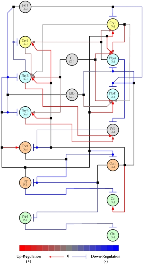
Illustration of Network Inference: The Predicted Pathway of the Circadian Regulatory System of Arabidopsis According to Chang et al. (2005). The network nodes (ovals) represent genes and are differentiated by color into cryptochrome (yellow), phytochrome (light blue), clock genes (orange), light-dependent downstream genes (light green), and other relevant genes (gray). The edges (lines) represent inferred causal relationships in a spectrum between activation (red) and repression (blue). Edges corresponding to activation are additionally marked by terminating arrows, and inhibitory edges are marked by terminating blunt segments. Combinatorial regulation is indicated by edge junctions shown as filled squares or circles. A filled square attached to a line indicates where an edge starting from a regulatory node bifurcates to affect several downstream nodes. A filled circle attached to a line indicates the case when several upstream nodes regulate the same target node. Figure reproduced from Chang et al. (2005).

Illustration of Predictions from a Discrete Dynamic Model: The Percentage of Simulated Stomata That Attain ABA-Induced Closure as a Function of Time Steps in Li et al. (2006). This Boolean model circumvents the lack of information in the timing of each process, in the internal states of signaling proteins, and in the concentrations of small molecules by performing a large number of simulations that sample equally over relative durations and node initial states. The results are reported as the percentage of simulations that attain the on state for the node closure. In all panels, black triangles with dashed lines signify the model's representation of normal (wild-type) response to ABA stimulus. Open triangles with dashed lines show that in the wild type, the percentage of closed simulated stomata decays in the absence of ABA. (A) The model predicts that disruption of depolarization (open diamonds) or anion efflux at the plasma membrane (open squares) cause total loss of ABA-induced closure. (B) The model predicts that perturbations in sphingosine-1-phosphate (dashed squares), phosphatidic acid (dashed circles), or pHc (dashed diamonds) lead to reduced closure probability. (C) The model predicts that abi1 recessive mutants (black squares) show faster than wild-type ABA-induced closure (ABA hypersensitivity). Blocking Cac2+ increase (black diamonds) causes slower than wild-type ABA-induced closure (ABA hyposensitivity) in the model. Figure reproduced from Li et al. (2006).
References
-
- Agrawal, V., Zhang, C., Shapiro, A.D., and Dhurjati, P.S. (2004). A dynamic mathematical model to clarify signaling circuitry underlying programmed cell death control in Arabidopsis disease resistance. Biotechnol. Prog. 20 426–442. - PubMed
-
- Albert, I., and Albert, R. (2004). Conserved network motifs allow protein-protein interaction prediction. Bioinformatics 20 3346–3352. - PubMed
-
- Albert, R., and Barabási, A.L. (2002). Statistical mechanics of complex networks. Rev. Mod. Phys. 74 47–97.
-
- Albert, R., DasGupta, B., Dondi, R., Kachalo, S., Sontag, E., Zelikovsky, A., and Westbrooks, K. (2007. a). A novel method for signal transduction network inference from indirect experimental evidence. J. Comput. Biol. 14 927–949. - PubMed
-
- Albert, R., DasGupta, B., Dondi, R., Kachalo, S., Sontag, E.D., Zelikovsky, A., and Westbrook, K. (2007. b). A novel method for signal transduction network inference from indirect experimental evidence. J. Comput. Biol. 14 927–949. - PubMed
Publication types
MeSH terms
LinkOut - more resources
Full Text Sources
Other Literature Sources
