The diffusion decision model: theory and data for two-choice decision tasks

Abstract

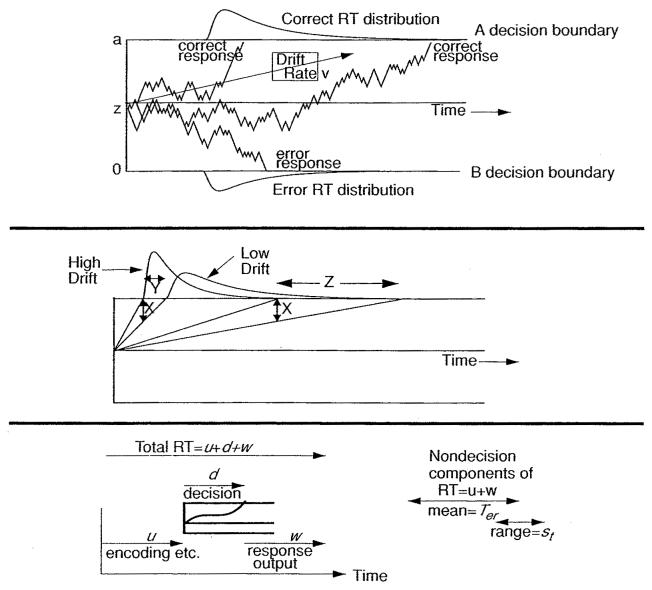
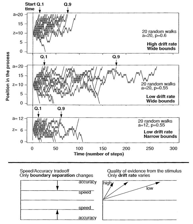
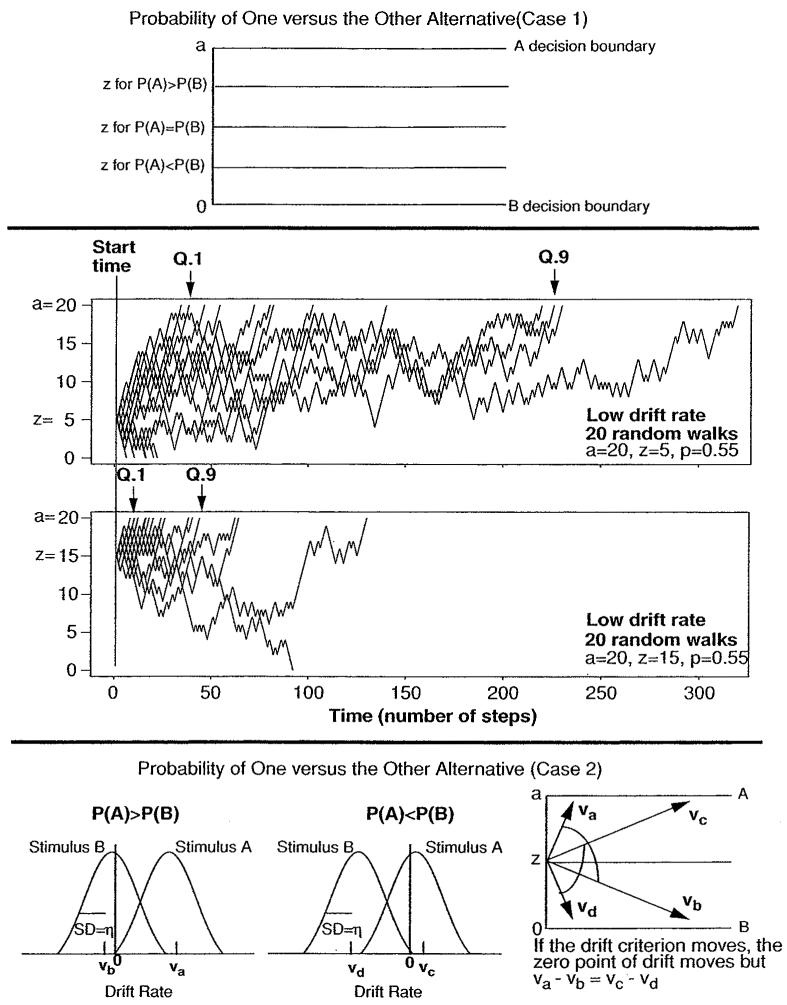
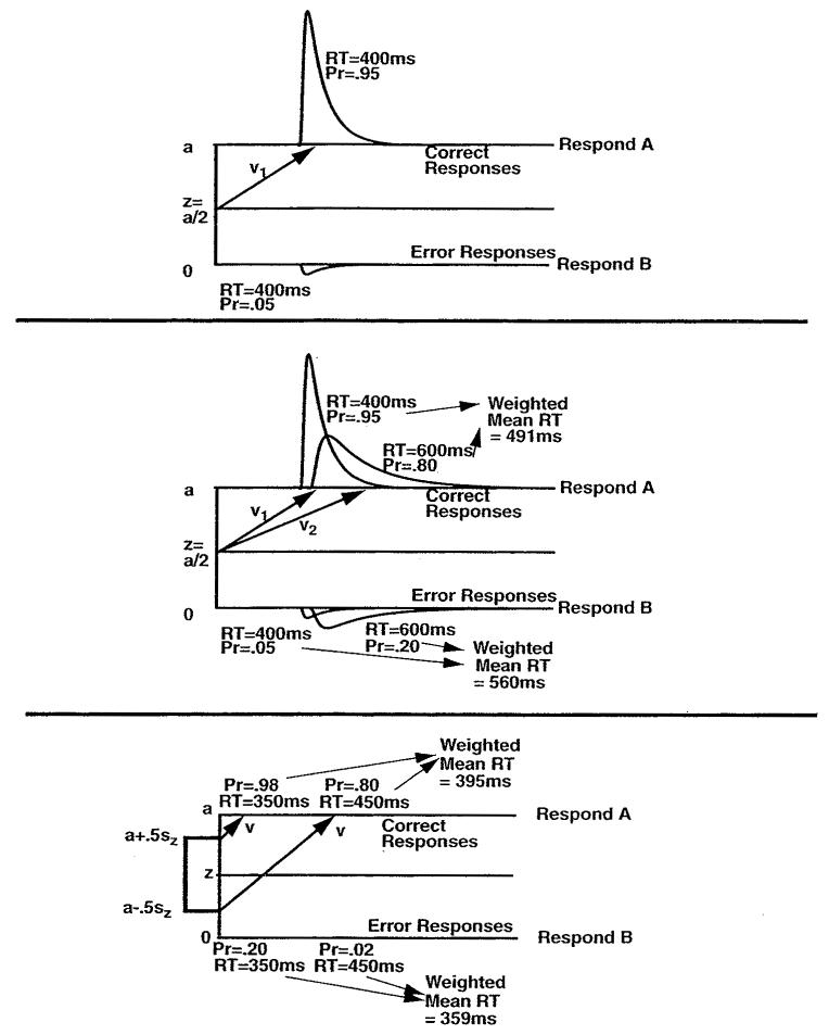
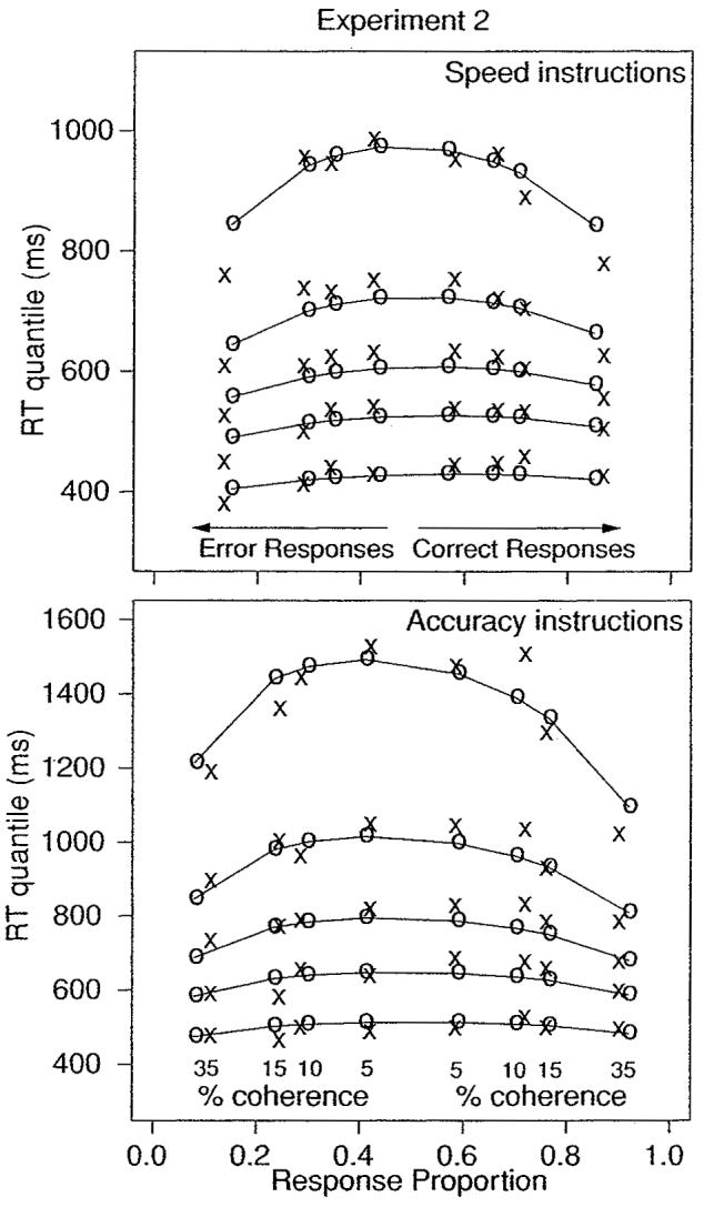
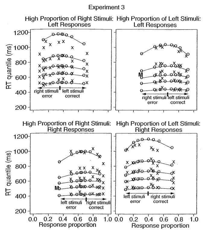
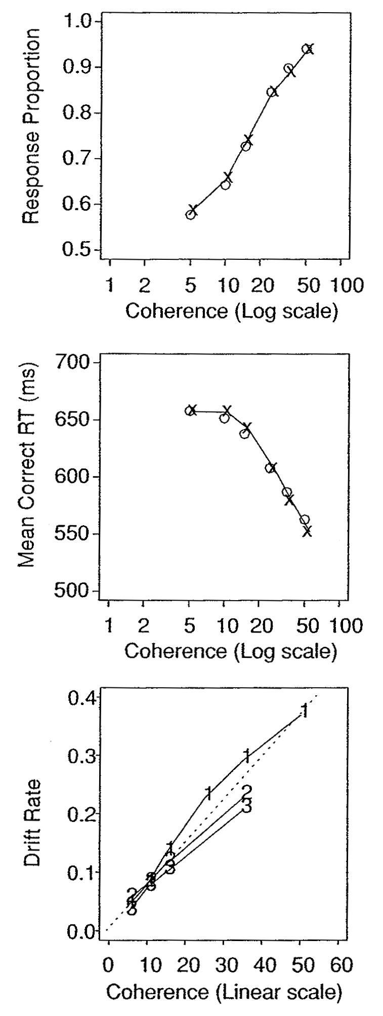
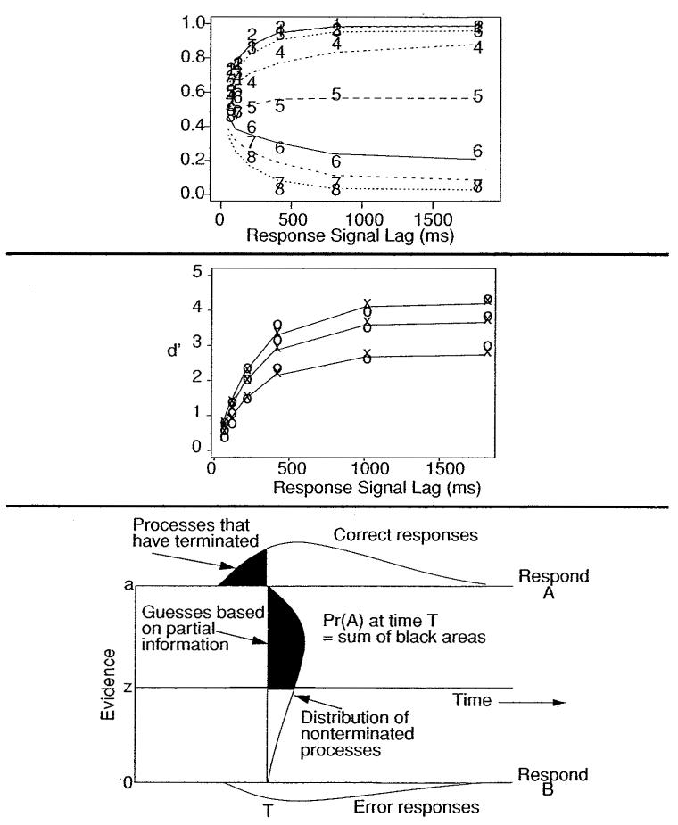
The diffusion decision model allows detailed explanations of behavior in two-choice discrimination tasks. In this article, the model is reviewed to show how it translates behavioral data-accuracy, mean response times, and response time distributions-into components of cognitive processing. Three experiments are used to illustrate experimental manipulations of three components: stimulus difficulty affects the quality of information on which a decision is based; instructions emphasizing either speed or accuracy affect the criterial amounts of information that a subject requires before initiating a response; and the relative proportions of the two stimuli affect biases in drift rate and starting point. The experiments also illustrate the strong constraints that ensure the model is empirically testable and potentially falsifiable. The broad range of applications of the model is also reviewed, including research in the domains of aging and neurophysiology.

Figure 1

The diffusion decision model. (Top panel) Three simulated paths with drift rate v, boundary separation a, and starting point z. (Middle panel) Fast and slow processes from each of two drift rates to illustrate how an equal size slowdown in drift rate (X) produces a small shift in the leading edge of the RT distribution (Y) and a larger shift in the tail (Z). (Bottom panel) Encoding time (u), decision time (d), and response output (w) time. The nondecision component is the sum of u and w with mean = T_er and with variability represented by a uniform distribution with range s_t.

Figure 2

Simulated diffusion processes. Each of the top three panels shows 20 processes simulated by random walks. Q.1 and Q.9 refer to the .1 and .9 quantiles of the resulting sets of RTs. For the top simulation, the upper boundary is a = 20 (the starting point is z = a/2 in each simulation), the lower boundary is 0, and the probability of taking a step toward the top boundary of .6. For the second simulation, the probability of taking a step toward the top boundary is reduced to .55, and for the third simulation, the upper boundary is reduced to a = 12. On the bottom panel, boundary separation alone changes between speed and accuracy instructions, and drift rate alone varies with stimulus difficulty.

Figure 3

Diffusion model explanations for the effects of response probability manipulations. In the top panel, the first possible account is presented: starting point varying with probability. The effects are illustrated with two simulations in the second panel with z = 5 and z = 15. In the bottom panel, the second possibility is presented: drift criterion (the zero point) varying with probability. When the probability of response A is higher, the drift rates are v_a and v_b, with the zero point close to v_b. When the probability of response B is higher, the drift rates are v_c and v_d, and the zero point is closer to v_c. Note that this second alternative is exactly equivalent to how the criterion would change in signal detection theory from psychophysics.

Figure 4

Variability in drift rate and starting point and the effects on speed and accuracy. The top panel shows RT distributions and response probabilities for correct and error responses with drift rate v. For a single drift rate, correct and error responses have equal RTs, 400 ms in the illustration. The middle panel shows two process with drift rates v₁ and v₂ and the starting point halfway between the boundaries with correct and error RTs of 400 ms for v₁ and 600 ms for v₂. Averaging these two illustrates the effects of variability in drift rate across trials and in the illustration yields error responses slower than correct responses. The bottom panel shows processes with two starting points and drift rate v. Averaging processes with starting point a + .5s_z (high accuracy and short RTs) and starting point a − .5s_z (lower accuracy and short RTs) yield error responses faster than correct responses.

Figure 5

A RT distribution overlaid with .1, .3, .5, .7, and .9 quantiles, where the .1 quantile ranges from .005 to .1 and the .9 quantile from .9 to .995. The areas between each pair of middle quantiles are .2, and the areas below .1 and above .9 are .095. The quantile rectangles capture the main features of the RT distribution and therefore a reasonable summary of overall distribution shape.

Figure 6

Quantile probability functions. The figures show possible outcomes for experiment 1 in which there are six levels of coherence (from 5% to 50%). Predicted quantile RTs for the .1, .3, .5 (median), .7, and .9 quantiles (stacked vertically) are plotted against response proportion for each of the six conditions. Correct responses for left- and right-moving stimuli, combined, are plotted to the right, and error responses for left- and right-moving stimuli combined are plotted to the left. The bold horizontal line in each figure connects correct and error median RTs for the third most accurate condition in order to highlight whether error responses are slower or faster than correct responses. The drift rates from which the data were simulated are those obtained in experiment 1. For all six panels, the starting point (z) was halfway between the boundaries. Across the six panels, boundary separation a takes on values of 0.16, 0.11, or 0.08; across-trial variability in starting point rate s_z takes on values of 0 or 0.07; across-trial variability in T_er, s_t, takes on values of 0 or 0.20; and across-trial variability in drift rate, η, takes on values of 0 or 0.12. T_er is the mean time taken up by the nondecision components of processing is set at 300 ms in the plots.

Figure 7

Quantile probability functions for experiment 1.

Figure 8

Quantile RTs for the six conditions in experiment 1 plotted against quantiles for the third most accurate condition (25% coherence). The top panel shows data quantiles, and the bottom panel shows quantiles predicted from the diffusion model.

Figure 9

Quantile probability functions for the speed and accuracy instruction conditions for experiment 2.

Figure 10

Quantile probability functions for high- and low-proportion stimuli for experiment 3.

Figure 11

Response proportion, mean RT for correct responses, and drift rate as a function of coherence. For the top and middle panels, the o's are data, and the x's are predictions from the diffusion model. In the bottom panel, the numerals 1, 2, and 3 refer to experiments 1, 2, and 3.

Figure 12

The response signal procedure, data, and diffusion model explanations. The top panel shows response proportion as a function of response signal lag from a numerosity discrimination experiment (Ratcliff, 2006) in which subjects judged whether the number of dots in a 10 × 10 array was greater than 50 or less or equal to 50. The eight lines represent eight groupings of numbers of dots (e.g., 13–20, 21–30, 31–40, 41–50, 51–60, 61–70, 71–80, and 81–87 dots). The middle panel shows d′ increasing as a function of lag for three well-separated positive conditions, where d′ is the difference in z-scores between each of the three conditions and a baseline condition (condition 6 from the top panel). The bottom panel shows how the diffusion model accounts for response signal data. The proportion of A responses at time T is the sum of processes that have terminated at the A boundary (the black area above the boundary) and nonterminated processes (the black area still within the diffusion process).

References

1. Ashby FG. A stochastic version of general recognition theory. Journal of Mathematical Psychology. 2000;44:310–329. - PubMed
1. Ball K, Sekuler R. A specific and enduring improvement in visual motion discrimination. Science. 1982;218:697–698. - PubMed
1. Bogacz R, Brown E, Moehlis J, Holmes P, Cohen JD. The physics of optimal decision making: A formal analysis of models of performance in two-alternative forced choice tasks. Psychological Review. 2006;113:700–765. - PubMed
1. Britten KH, Shadlen MN, Newsome WT, Movshon JA. The analysis of visual motion: A comparison of neuronal and psychophysical performance. Journal of Neuroscience. 1992;12:4745–4765. - PMC - PubMed
1. Buchanan L, McEwen S, Westbury C, Libben G. Semantics and semantic errors: Implicit access to semantic information from words and nonwords in deep dyslexia. Brain and Language. 2003;84:65–83. - PubMed
Publication types