The properties of high-dimensional data spaces: implications for exploring gene and protein expression data

Abstract

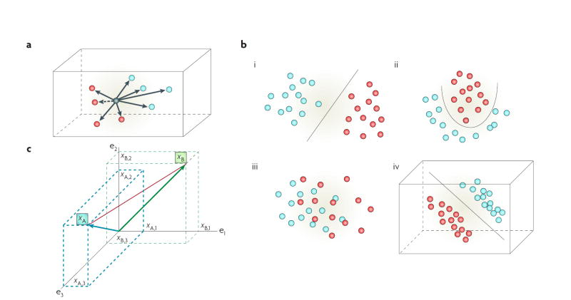
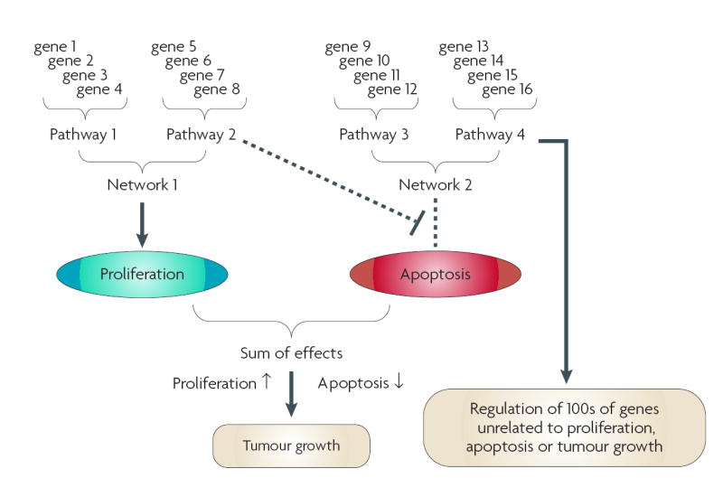
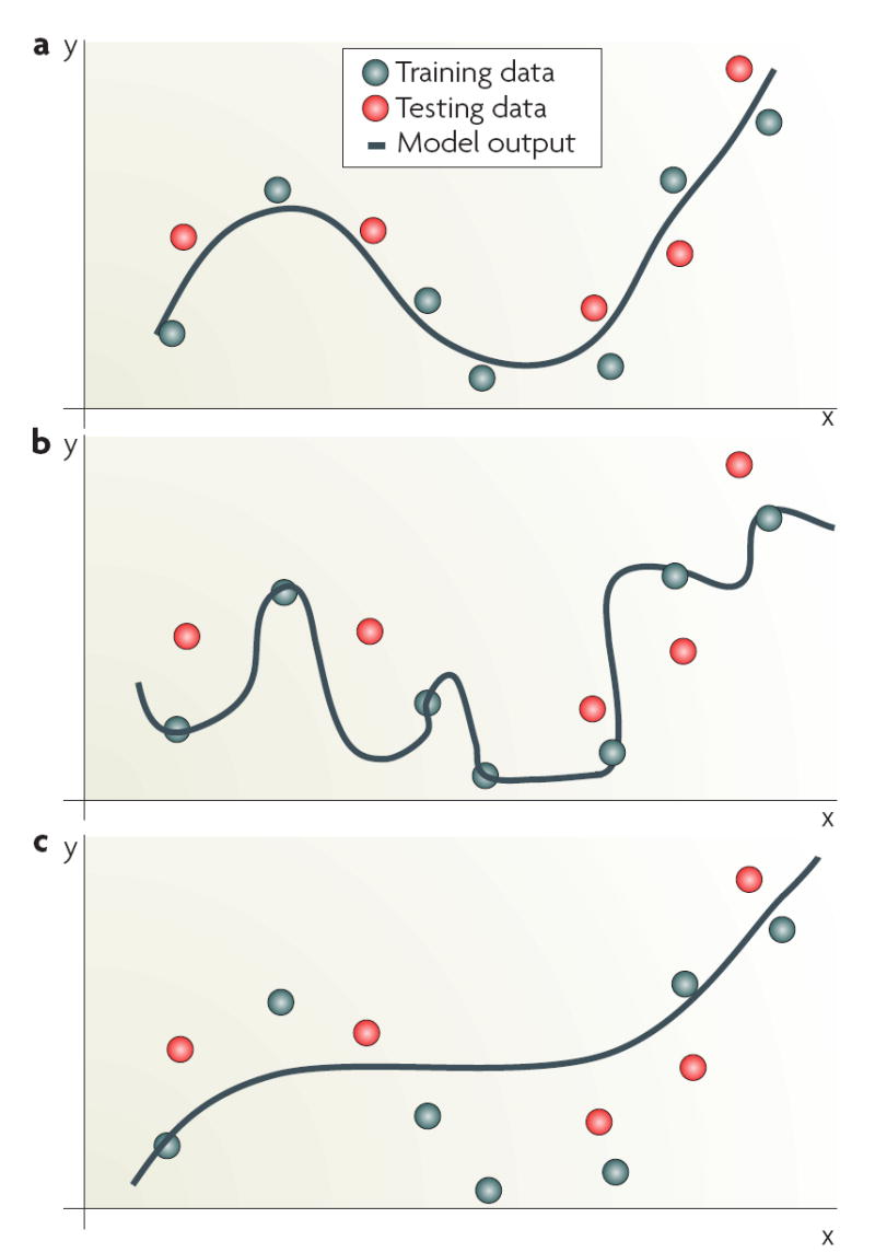
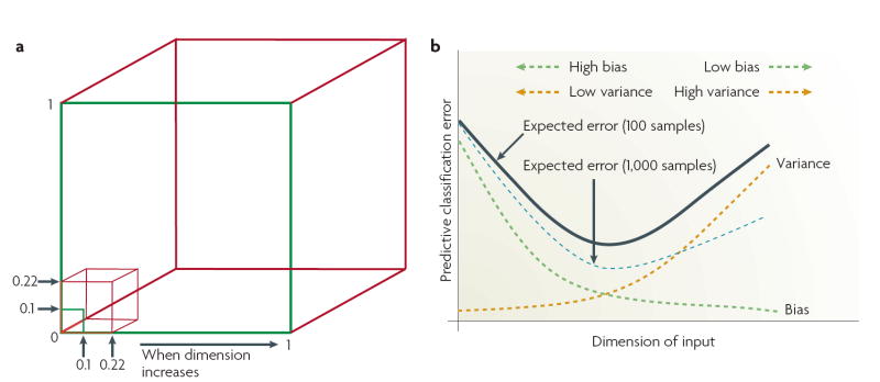
High-throughput genomic and proteomic technologies are widely used in cancer research to build better predictive models of diagnosis, prognosis and therapy, to identify and characterize key signalling networks and to find new targets for drug development. These technologies present investigators with the task of extracting meaningful statistical and biological information from high-dimensional data spaces, wherein each sample is defined by hundreds or thousands of measurements, usually concurrently obtained. The properties of high dimensionality are often poorly understood or overlooked in data modelling and analysis. From the perspective of translational science, this Review discusses the properties of high-dimensional data spaces that arise in genomic and proteomic studies and the challenges they can pose for data analysis and interpretation.

Figure 1. Cluster separability in data space

a | Each data point exists in the space defined by its attributes and by its relative distance to all other data points. The nearest neighbour (dashed arrow) is the closest data point. The goal of clustering algorithms is to assign the data point to membership in the most appropriate cluster (red or blue cluster). Many widely used analysis methods force samples to belong to a single group or link them to their estimated nearest neighbour and do not allow concurrent membership of more than one area of data space (hard clustering; such as k-means clustering or hierarchical clustering based on a distance matrix). Analysis methods that allow samples to belong to more than one cluster (soft clustering; such as that using the expectation-maximization algorithm) may reveal additional information. b | Data classes can be linearly separable or non-linearly separable. When linearly separable, a linear plane can be found that separates the data clusters (i). Non-linearly separable data can exist in relatively simple (ii) or complex (iii) data space. Well-defined clusters in simple data space may be separated by a non-linear plane (ii). In complex data space, cluster separability may not be apparent in low-dimensional visualizations (iii), but may exist in higher dimensions (iv). c | Expression data can be represented as collections of continuously valued vectors, each corresponding to a sample’s gene-expression profile. Data are often arranged in a matrix of N rows (samples) and D columns (variables or genes). The distance of a data point to the origin (vector space), or the distance between two data points (metric space), is defined by general mathematical rules. A (blue arrow) and B (green arrow) are vectors and their Euclidean distance is indicated by the red line. Individual data points, each represented by a vector, can form clusters, as in the examples of two clusters in b.

Figure 2. High dimensional expression data are multimodal

Most univariate and multivariate probability theories were derived for data space where N (number of samples) > D (number of dimensions). Expression data are usually very different (D>>>N). A study of 100 mRNA populations (one from each of 100 tumours) arrayed against 10,000 genes can be viewed as each of the 100 tumours existing in 10,000-D space. This data structure is the inverse of an epidemiological study of 10,000 subjects (samples) for which there are data from 100 measurements (dimensions), yet both data sets contain 10⁶ data points. A further concern arises from the multimodal nature of high-dimensional data spaces. The dynamic nature of cancer and the concurrent activity of multiple biological processes occurring within the microenvironment of a tumour create a multimodal data set. Genes combine into pathways; pathways combine into networks. Genes, pathways and/or networks interact to affect subphenotypes (proliferation, apoptosis); subphenotypes contribute to clinically relevant observations (tumour size, proliferation rate). Genes in pathway 2 are directly associated with a network (and with pathway 1) and a common subphenotype (increased proliferation). Genes in pathway 2 are also inversely associated with a subphenotype (apoptosis). Here, multimodality captures the complex redundancy and degeneracy of biological systems and the concurrent expression of multiple components of a complex phenotype. For example, tumour growth reflects the balance between cell survival, proliferation and death, and cell loss from the tumour (such as through invasion and metastasis), each being regulated by a series of cellular signals and functions. Many such complex functions may coexist, such as growth-factor or hormonal stimulation of tumour cell survival or proliferation, or the ability to regulate a specific cell-death cascade. A molecular profile from a tumour may contain subpatterns of genes that reflect each of these individual characteristics. This multimodality may be problematic for statistical modelling to build either accurate cell signalling networks or robust classification schemes.

Figure 3. Model fitting, dimensionality and the blessings of smoothness

a | Output of a smooth function that yields good generalization on previously unseen inputs. b | A model that performs well on the training data used for model building, but fails to generalize on independent data and is hence overfitted to the training data. c | A model that is insufficiently constructed and trained and is considered to be underfitted. The imposition of stability on the solution can reduce overfitting by ensuring that the function is smooth, and some random fluctuations are well-controlled in high-dimensions. This allows new samples that are similar to those in the training set to be similarly labelled. This phenomenon is often referred to as the ‘blessing of smoothness’. Stability can also be imposed using regularization that ensures smoothness by constraining the magnitude of the parameters of the model. Support vector machines apply a regularization term that controls the model complexity and makes it less likely to overfit the data (BOX 3). By contrast, k-nearest neighbour or weighted voting average algorithms overcome the challenge simply by reducing data dimensionality. Validation of performance is a crucial component in model building. Although an iterative sequential training is often used for both training and optimization, validation must be done using an independent data set (not used for model training or optimization) and where there are adequate outcomes relative to the number of variables in the model. For early proof-of-principle studies, for which an independent data set may not be available, some form of cross-validation can be used. For example, three-fold cross-validation is common, in which the classifier is trained on two-thirds of the overall data set and tested for predictive power on the other third,,. This process is repeated multiple times by reshuffling the data and re-testing the classification error.

Figure 4. The curse of dimensionality and the bias or variance dilemma

a | The geometric distributions of data points in low- and high-dimensional space differ significantly. For example, using a subcubical neighbourhood in a 3-dimensional data space (red cube) to capture 1% of the data to learn a local model requires coverage of 22% of the range of each dimension (0.01 ≈ 0.22³) as compared with only 10% coverage in a 2-dimensional data space (green square) (0.01 = 0.10²). Accordingly, using a hypercubical neighbourhood in a 10-dimensional data space to capture 1% of the data to learn a local model requires coverage of as much as 63% of the range of each dimension (0.01 ≈ 0.63¹⁰). Such neighbourhoods are no longer ‘local’. As a result, the sparse sampling in high dimensions creates the empty space phenomenon: most data points are closer to the surface of the sample space than to any other data point. For example, with 5,000 data points uniformly distributed in a 10-dimensional unit ball centred at the origin, the median distance from the origin to the nearest data point is approximately 0.52 (more than halfway to the boundary), that is, a nearest-neighbour estimate at the origin must be extrapolated or interpolated from neighbouring sample points that are effectively far away from the origin. b | A practical demonstration is the bias–variance dilemma,,. Specifically, the mismatch between a model and data can be decomposed into two components; bias that represents the approximation error, and variance that represents the estimation error. Added dimensions can degrade the performance of a model if the number of training samples is small relative to the number of dimensions. For a fixed sample size, as the number of dimensions is increased there is a corresponding increase in model complexity (increase in the number of unknown parameters), and a decrease in the reliability of the parameter estimates. Consequently, in the high-dimensional data space there is a trade-off between the decreased predictor bias and the increased prediction uncertainty,.

Figure 5. Dimensionality reduction

A practical implication of the curse of dimensionality is that, when confronted with a limited training sample, an investigator will select a small number of informative features (variables or genes). A supervised method can select these features (reduce dimensionality), where the most useful subset of features (genes or proteins) is selected on the basis of the classification performance of the features. The crucial issue is the choice of a criterion function. Commonly used criteria are the classification error and joint likelihood of a gene subset, but such criteria cannot be reliably estimated when data dimensionality is high. One strategy is to apply bootstrap re-sampling to improve the reliability of the model parameter estimates. Most approaches use relatively simple criterion functions to control the magnitude of the estimation variance. An ensemble approach can be derived, as multiple algorithms can be applied to the same data with embedded multiple runs (different initializations, parameter settings) using bootstrap samples and leave-one-out cross-validation. Stability analysis can then be used to assess and select the converged solutions. Unsupervised methods such as principal component analysis (PCA) can transform the original features into new features (principal components (PC)), each PC representing a linear combination of the original features. PCA reduces input dimensionality by providing a subset of components that captures most of the information in the original data. For example, those genes that are highly correlated with the most informative PCs could be selected as classifier inputs, rather than a large dimension of original variables containing redundant features,. Non-linear PCA, such as kernel PCA can also be used for dimensionality reduction but adds the capability, through kernel-based feature spaces, to look for non-linear combinations of the input variables. PCA is useful for classification studies but is potentially problematic for molecular signalling studies. If PC1 is used to identify genes that are differentially expressed between phenotypes 1 and 2, then genes that are strongly associated with PC1 (black circles) would be selected. If both PC1 and PC2 are used, then genes strongly associated with PC1 (black circles) and PC2 (blue circles) would be selected. Some genes could be differentially expressed but weakly associated with the top two PCs (PC1, PC2) and so not selected (red circles). As their rejection is not based on biological function(s), key mechanistic information could be lost.

References

1. Khan J, et al. Classification and diagnostic prediction of cancers using gene expression profiling and artificial neural networks. Nature Med. 2001;7:673–679. Example of the successful use of molecular profiling to improve cancer diagnosis.
1. Bhanot G, Alexe G, Levine AJ, Stolovitzky G. Robust diagnosis of non-Hodgkin lymphoma phenotypes validated on gene expression data from different laboratories. Genome Inform. 2005;16:233–244. - PubMed
1. Lin YH, et al. Multiple gene expression classifiers from different array platforms predict poor prognosis of colorectal cancer. Clin Cancer Res. 2007;13:498–507. - PubMed
1. Lopez-Rios F, et al. Global gene expression profiling of pleural mesotheliomas: overexpression of aurora kinases and P16/CDKN2A deletion as prognostic factors and critical evaluation of microarray-based prognostic prediction. Cancer Res. 2006;66:2970–2979. - PubMed
1. Ganly I, et al. Identification of angiogenesis/ metastases genes predicting chemoradiotherapy response in patients with laryngopharyngeal carcinoma. J Clin Oncol. 2007;25:1369–1376. - PubMed
Publication types