Origin and dynamics of extraclassical suppression in the lateral geniculate nucleus of the macaque monkey

Abstract

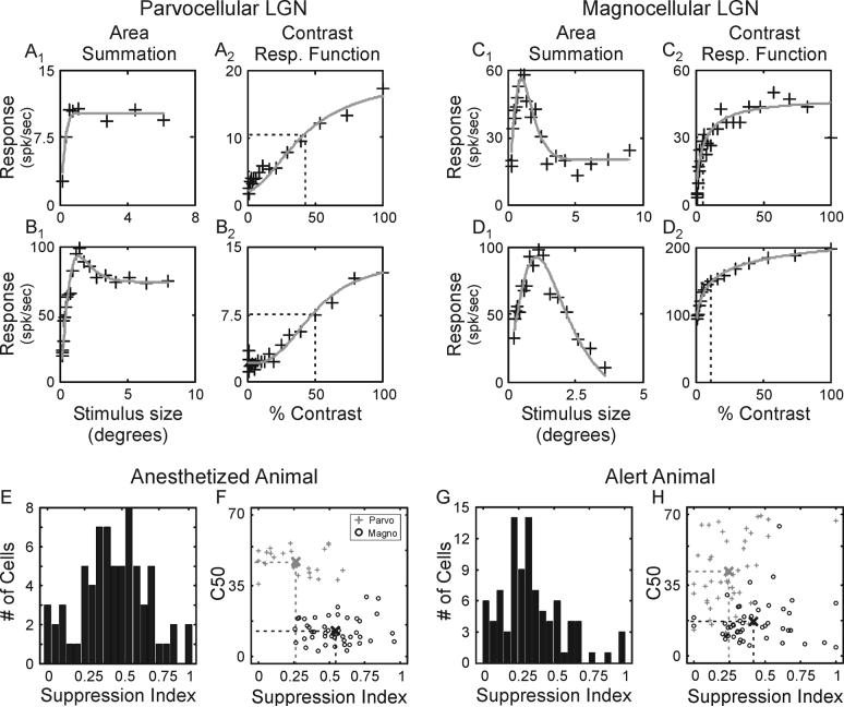
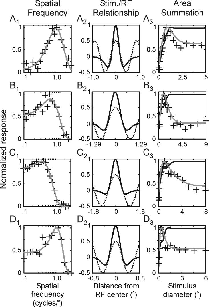
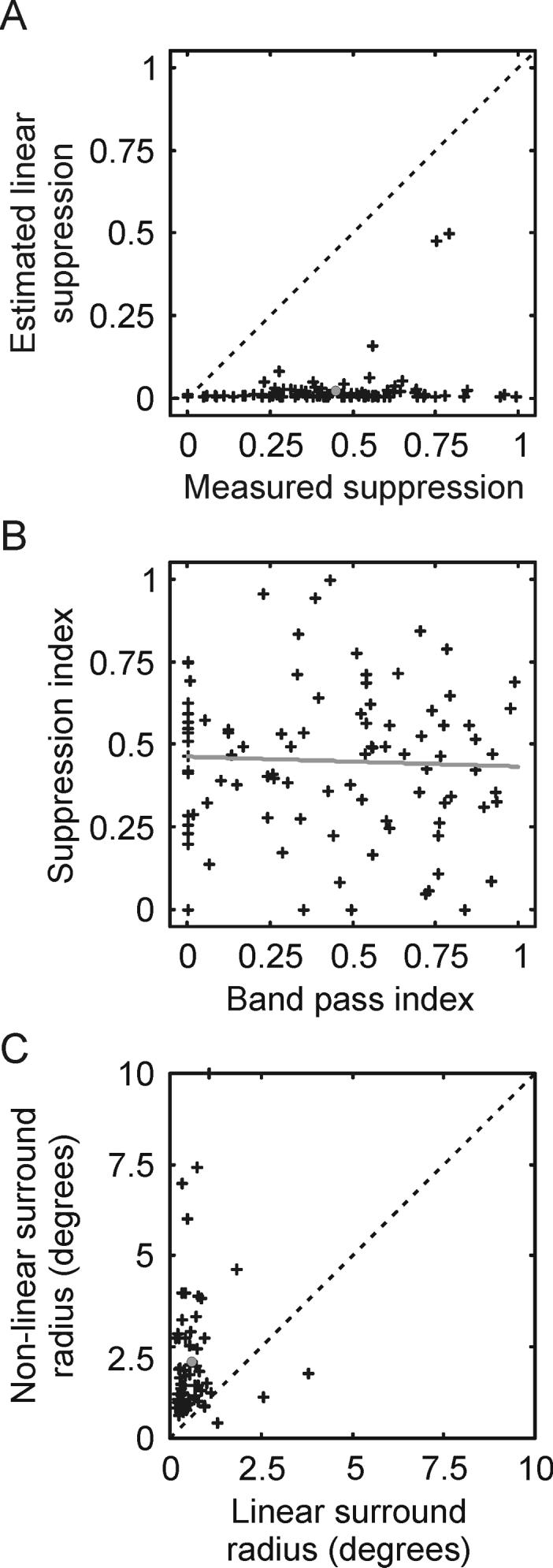
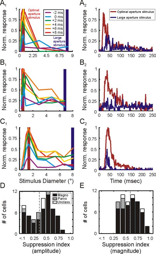
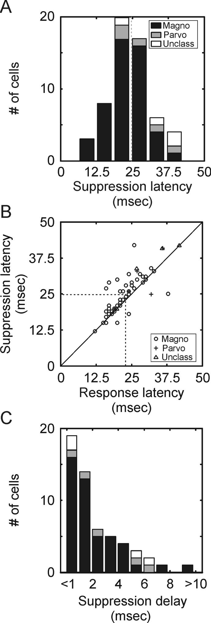
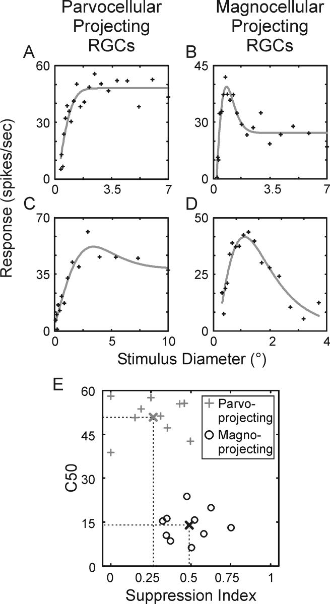
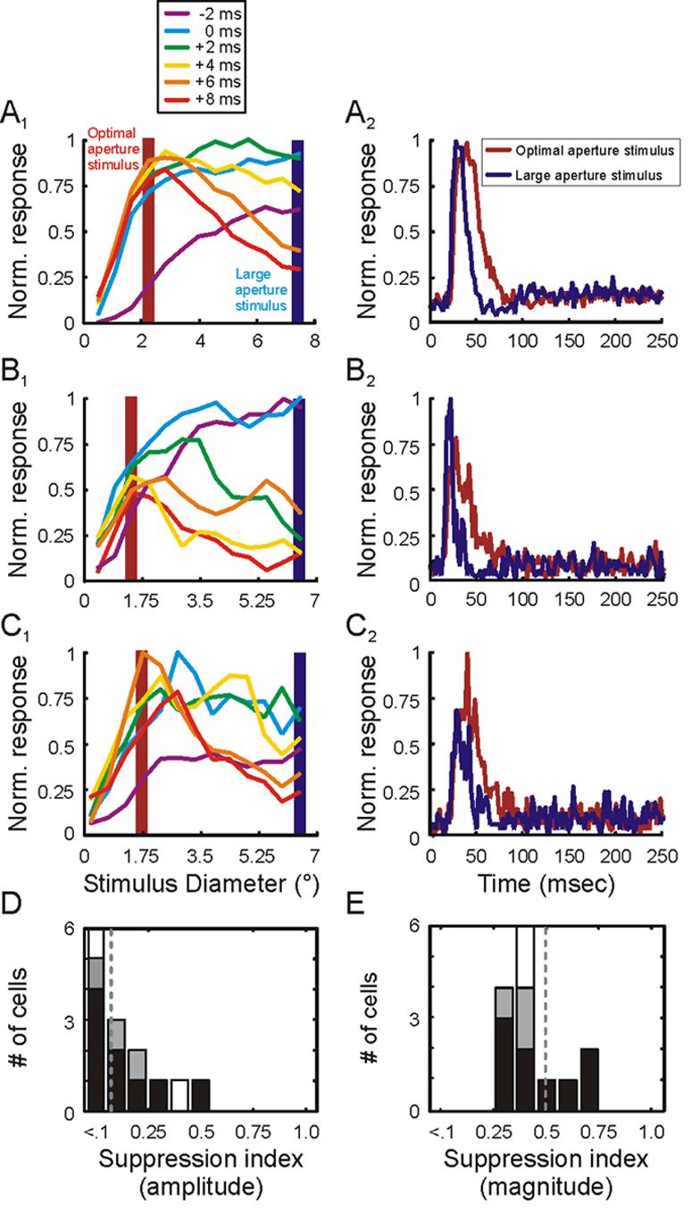
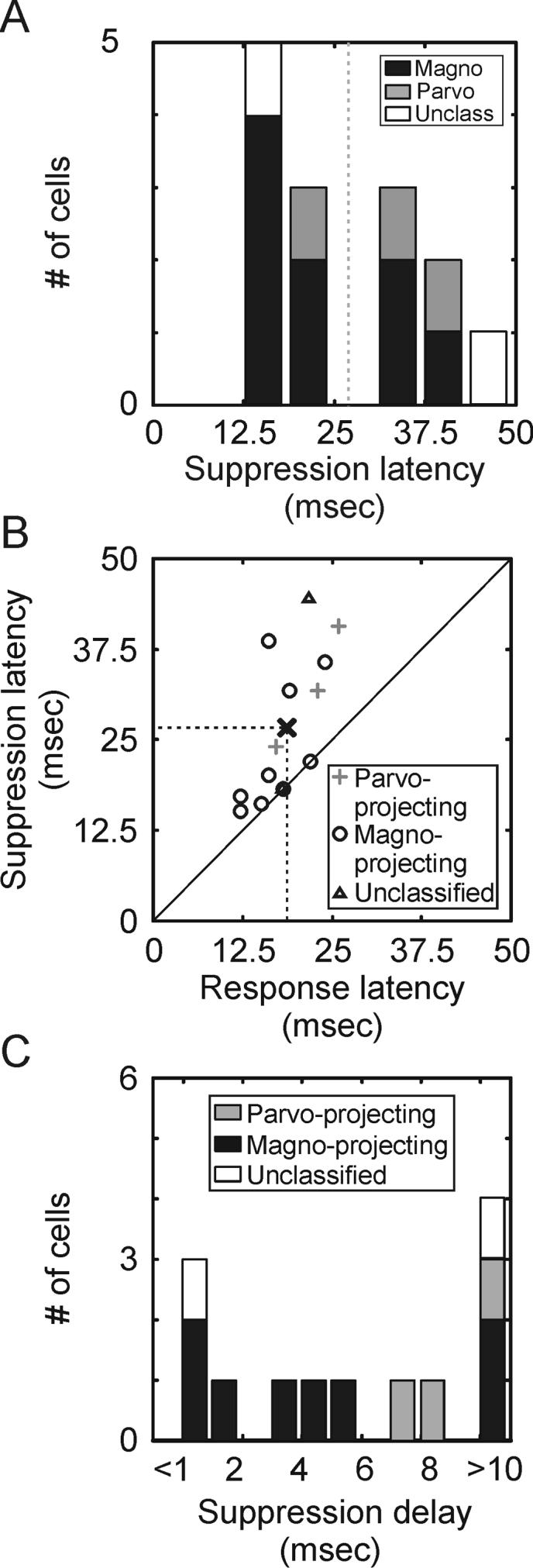
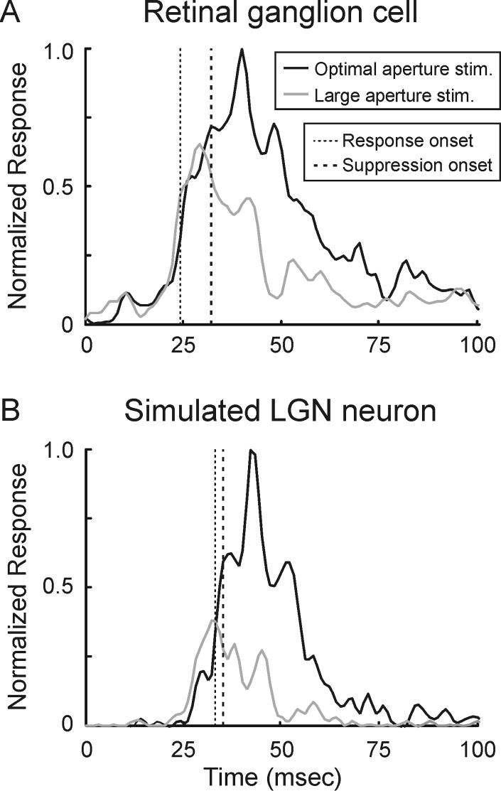
In addition to the classical, center/surround receptive field of neurons in the lateral geniculate nucleus (LGN), there is an extraclassical, nonlinear surround that can strongly suppress LGN responses. This form of suppression likely plays an important role in adjusting the gain of LGN responses to visual stimuli. We performed experiments in alert and anesthetized macaque monkies to quantify extraclassical suppression in the LGN and determine the roles of feedforward and feedback pathways in the generation of LGN suppression. Results show that suppression is significantly stronger among magnocellular neurons than parvocellular neurons and that suppression arises too quickly for involvement from cortical feedback. Furthermore, the amount of suppression supplied by the retina is not significantly different from that in the LGN. These results indicate that extraclassical suppression in the macaque LGN relies on feedforward mechanisms and suggest that suppression in the cortex likely includes a component established in the retina.

Figure 1

Area summation tuning properties of LGN neurons in the macaque monkey. A-D. Area summation tuning curves and contrast response functions for 2 representative parvocellular neurons and 2 representative magnocellular neurons. Area summation tuning curves (A₁, B₁, C₁, D₁) were fitted to a spatial domain difference of Gaussians (DOG_S) equation (gray line); contrast response functions (A₂, B₂, C₂, D₂) were fitted to a hyperbolic ratio (gray line). Dashed lines in the contrast response functions show the contrast to evoke a half-maximum response (C50). E and G. Distribution of suppression index values across LGN neurons in anesthetized and alert animals. F and H. Scatter plots showing the relationship between suppression index and C50 across cells in anesthetized and alert animals. Sample means are indicated by crosses located at the intersections of the two dashed lines.

Figure 2

Estimating the contribution of linear suppression to area summation tuning curves. A₁, B₁, C₁, D₁. Spatial frequency tuning curves from 4 representative neurons fitted to a frequency-domain difference of Gaussians (DOG_f) equation (lines). A₂, B₂, C₂, D₂. DOG receptive field profiles of the 4 representative neurons (dark lines) along with the luminance profiles of the sine-wave gratings used in the area summation experiments (dashed gray lines). A₃, B₃, C₃, D₃. Estimated area summation tuning curves based on the classical receptive fields of the 4 representative neurons (dark lines) along with their measured tuning curves (gray lines).

Figure 3

Relationship between the classical surround and extraclassical surround of LGN neurons. A. Scatter plot comparing suppression index values calculated from estimates of the linear contribution to suppression coming from the classical receptive field to actual suppression index values measured from area summation tuning curves. B. Scatter plot comparing extraclassical surround strength to classical surround strength. Extraclassical surround strength is quantified using a suppression index calculated from area summation tuning curves; classical surround strength is quantified using a band-pass index calculated from spatial frequency tuning curves. The dashed line shows the linear regression of the two values across cells. C. Comparison of the spatial size of the extraclassical receptive field with the size of the classical receptive field.

Figure 4

Temporal dynamics of area summation in the LGN. A₁, B₁, C₁. Area summation tuning curves for 3 representative neurons at 6 different relative times. The time when cells reached 25% of maximum response is defined as 0 msec. Each of the colored curves represents responses at times relative to 0 msec. Shaded red and blue bars highlight responses to optimal-size stimuli and large stimuli, respectively. A₂, B₂, C₂. Time course of responses to optimal-size stimuli (red traces) and large stimuli (blue traces) for the 3 representative neurons. D and E. Distribution of suppression index values using amplitude (D) and magnitude (E) measures from each cell's area summation tuning curve. Magnocellular neurons represented in black, parvocellular neurons represented in gray, unclassified neurons represented in white.

Figure 5

Suppression latency in the LGN. A. Distribution of suppression latencies across the sample of LGN neurons. Suppression latency is defined as the time when responses to optimal-size stimuli and large stimuli first reach 25% of the maximum difference. Magnocellular neurons represented in black, parvocellular neurons represented in gray, unclassified neurons represented in white. This analysis is restricted to neurons with at least 30% suppression. B. Scatter plot showing the relationship between response latency and suppression latency. Response latency is defined as the earliest time that responses reached 25% of maximum response. Suppression latency is defined as described in A. C. Distribution of delays between the response latency and suppression latency across the sample of neurons.

Figure 6

Area summation tuning properties of retinal ganglion cells in the macaque monkey. A and C. Area summation tuning curves from 2 representative parvocellular-projecting ganglion cells. Tuning curves were fitted to a spatial domain difference of Gaussians (DOG_S) equation (gray line). B and D. Area summation tuning curves from 2 representative magnocellular-projecting ganglion cells. E. Scatter plot showing the relationship between the suppression index and contrast to evoke a half-maximum response (C50) across cells. Parvocellular-projecting ganglion cells represented with gray crosses, magnocellular-projecting ganglion cells represented with black circles. Thick crosses indicate the means for the two samples.

Figure 7

Temporal dynamics of area summation in the retina. A₁, B₁, C₁. Area summation tuning curves for 3 representative retinal ganglion cells at 6 different relative times. The time when cells reached 25% of maximum response is defined as 0 msec. Each of the colored curves represents responses at times relative to 0 msec. Shaded red and blue bars highlight responses to optimal-size stimuli and large stimuli, respectively. A₂, B₂, C₂. Time course of responses to optimal-size stimuli (red traces) and large stimuli (blue traces) for the 3 representative ganglion cells. D and E. Distribution of suppression index values using amplitude (D) and magnitude (E) measures from each cell's area summation tuning curve. Magnocellular neurons represented in black, parvocellular neurons represented in gray, unclassified neurons represented in white.

Figure 8

Suppression latency of retinal ganglion cells. A. Distribution of suppression latencies across the sample of retinal ganglion cells. Suppression latency is defined as the time when responses to optimal-size stimuli and large stimuli first reach 25% of the maximum difference. Magnocellular neurons represented in black, parvocellular neurons represented in gray, unclassified neurons represented in white. This analysis is restricted to neurons with at least 30% suppression. B. Scatter plot showing the relationship between response latency and suppression latency. Response latency is defined as the earliest time that responses reached 25% of maximum response. Suppression latency is defined as described in A. C. Distribution of delays between the response latency and suppression latency across the sample of retinal ganglion cells.

Figure 9

Temporal dynamics of surround suppression in a model LGN neuron. A. Time course of responses measured from a retinal ganglion cell stimulated with an optimal-size stimulus (red trace) and a large stimulus (blue trace). The delay between response latency and suppression latency is 8 msec. B. Time course of responses from a modeled LGN neuron that received input from the cell in A. Spiking responses in the LGN neuron were generated by passing the retinal spike trains through an exponential filter (τ = 5 msec) with a spike threshold. For this model neuron, the delay between response latency and suppression latency is 1.5 msec.

References

1. Alonso J-M, Usrey WM, Reid RC. Rules of connection for neurons in the lateral geniculate nucleus and visual cortex. J. Neurosci. 2001;21:4002–4015. - PMC - PubMed
1. Angelucci A, Bressloff PC. Contribution of feedforward, lateral and feedback connections to the classical receptive field center and extra-classical receptive field surround of primate V1 neurons. Prog. Brain Res. 2006;154:93–120. - PubMed
1. Angelucci A, Sainsbury K. Contribution of feedforward thalamic afferents and corticogeniculate feedback to the spatial summation area of macaque V1 and LGN. J. Comp. Neurol. 2006;498:330–351. - PubMed
1. Bair W, Cavanaugh JR, Movshon JA. Time course and time-distance relationships for surround suppression in macaque V1 neurons. J. Neurosci. 2003;23:7690–701. - PMC - PubMed
1. Benardete EA, Kaplan E, Knight BW. Contrast gain control in the primate retina: P cells are not X-like, some M cells are. Vis. Neurosci. 1992;8:483–486. - PubMed
Publication types
LinkOut - more resources