

Review
doi: 10.1038/nrn2315.
Regulation of spike timing in visual cortical circuits
Affiliations
- PMID: 18200026
- PMCID: PMC2868969
- DOI: 10.1038/nrn2315
Item in Clipboard
Review
Regulation of spike timing in visual cortical circuits
Nat Rev Neurosci.
2008 Feb.
Abstract
A train of action potentials (a spike train) can carry information in both the average firing rate and the pattern of spikes in the train. But can such a spike-pattern code be supported by cortical circuits? Neurons in vitro produce a spike pattern in response to the injection of a fluctuating current. However, cortical neurons in vivo are modulated by local oscillatory neuronal activity and by top-down inputs. In a cortical circuit, precise spike patterns thus reflect the interaction between internally generated activity and sensory information encoded by input spike trains. We review the evidence for precise and reliable spike timing in the cortex and discuss its computational role.
Figures
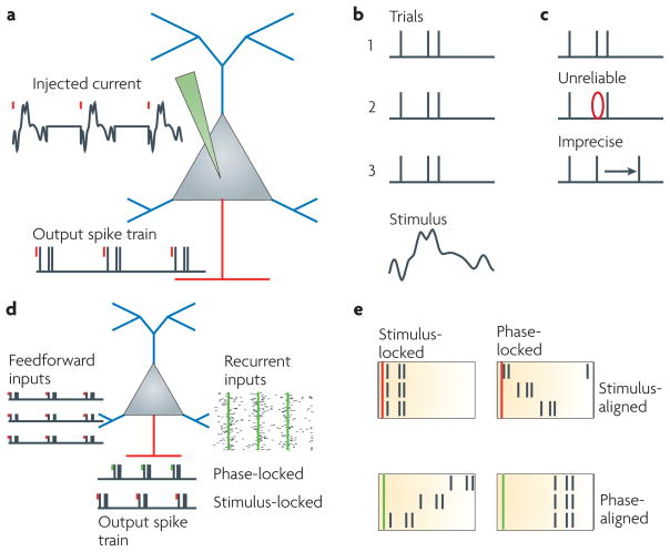
a| An in vitro reliability paradigm. A current consisting of many repeats of a short stimulus waveform followed by a period of zero current is injected using an electrode at the soma. The start of the stimulus is indicated by a red dash. The corresponding output spike train is shown at the bottom. b| Trials are aligned with the red dashes (the stimulus waveform is shown at the bottom). When the neuron is stimulus-locked, the spike trains are similar across trials. c| When spikes are missing in some trials but not in others, the neuron is considered unreliable. When the spike occurs but the spike time is variable, the neuron is considered imprecise (BOX 1). d| In vivo, the neuron receives feedforward inputs and recurrent inputs. When the same stimulus is presented repeatedly (represented by the red dashes), presynaptic neurons produce spike trains with repeatable motifs — spike patterns — that are similar in each neuron. Across a population, this input consists of a sequence of synchronized spike volleys. Recurrent inputs are periodic when the neuron is embedded in an oscillatory network. The beginning of each oscillation cycle is indicated by the green dashes. Two types of output spike train are shown: a stimulus-locked train and a phase-locked train. e| When the neuron is stimulus-locked, precise and reliable spike trains are obtained only when the trials are aligned with stimulus onset. When the neuron is phase-locked, precise and reliable spike trains emerge only when the spike trains are aligned with the start of the oscillation cycle.
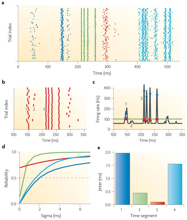
a| The spike trains shown were obtained from simulations of a model neuron with Hodgkin–Huxley-type voltage-gated channels driven by a fluctuating current. Similar trains could be obtained experimentally from neurons in vitro. The rastergram shown was constructed by plotting the spike train for each trial on a separate row, aligned with stimulus onset. The y ordinate of each tick is the trial number and the x ordinate is the spike time relative to the stimulus onset. For further analysis the data were divided into segments (shown in different colours). b| Twenty trials from part a from the time interval between 100 and 350 ms relative to the stimulus onset, showing that precision and reliability are distinct quantities. Event 1 is reliable — that is, a spike occurs on each trial — but it is not precise (there is a large jitter). Event 2 is precise but not reliable. Event 3 is both precise and reliable. c| Spike-time histogram, showing how the average firing rate (the number of spikes per second) across a series of trials changes with time. Events (blue stars) are peaks in the histogram and event reliability is the area under the peak. A threshold (the green line) is set, to define the events. When the threshold is set too high, unreliable events (such as event 2) are missed; when it is set too low, noise spikes could be interpreted as events. For the purpose of the reliability calculation (described in a previous publication; see REF. 135), each spike is replaced by a waveform of width sigma. The parameter sigma represents the temporal resolution of the spike times. d| Reliability as a function of sigma. Each curve is colour-coded to match the colour of the time segment in the rastergram (a) that was used in the calculation. The jitter (the standard deviation of the spike times in an event) corresponds approximately to the value of sigma for which the reliability becomes more than 0.5. The precision is equal to 1 divided by the jitter. e| The jitter for each segment. The third segment (shown in red) never intersects 0.5 and the jitter is not defined.
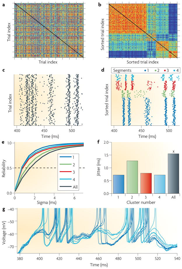
a,b| Having identified precise and reliable spike trains (see FIG. 2), spike patterns can be revealed. The value of the similarity (Sij) between the spike train on trial i and the spike train on trial j is represented as colour of the pixel on row i and column j. On the colour scale, blue indicates low similarity and red indicates high similarity. c,d| The rastergrams from which the similarity matrices in a and b, respectively, were calculated (the data were taken from the fourth segment (shown in cyan) of FIG. 2a). In a and c the trials are ordered as they are recorded, whereas in b and d they are reordered using fuzzy K-means clustering to bring similar trials close to each other. Spike patterns are operationally defined as groups of trials that are more similar to each other than to the other trials. In a no obvious structure is visible, but in b spike patterns have been uncovered. These patterns correspond to square blocks, with high similarity values on the diagonal. In d each spike pattern is shown in a different colour. The spike patterns had different spike times and, in some cases, a different number of spikes. e| Reliability is the average degree of similarity between pairs of spike trains at the temporal resolution given by the parameter sigma (BOX 1). Reliability is plotted against sigma for each spike pattern. f| The jitter (the standard deviation of the spike times in an event) for each spike pattern and across all trials. The precision (the inverse of the jitter) that is evaluated for each pattern separately is much higher than that which is calculated with all trials combined. g| Voltage traces corresponding to clusters 1 and 4. Cluster 4 spikes at 405 ms whereas cluster 1 does not; at 460 ms the situation is reversed. After a transient hyperpolarization that prevents spiking, the two voltage traces are close to convergence at 540 ms. This graph shows that spike patterns correspond to distinct voltage trajectories.
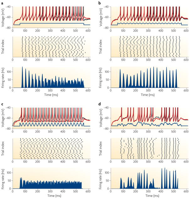
Each part shows, from top to bottom, a graph with two voltage traces (the red and black lines) and the stimulus waveform (the blue line), a rastergram and a histogram. The model neuron used in FIG. 2 provided the data. a| In response to a current step, precision decreases over time. b| When a periodic current is superimposed, the precision is maintained because of a resonance effect. The firing rate is approximately the same in a and b. c| When the phase of the periodic drive is varied from trial to trial the precision is reduced (the stimulus waveform is only shown for one phase). d| In response to an aperiodic current, well-defined events with a range of precisions are obtained.
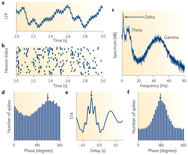
Phase locking to internal activity is uncovered by analysing simultaneously recorded spike trains and the local field potential (LFP) generated by a simple model. a| A short segment of an example LFP trace that was constructed by adding three noisy sinusoidal waveforms with frequencies in the gamma, theta and delta frequency ranges. b| Sample spike trains were constructed to be weakly phase-locked, in the gamma frequency range and at a delay of 50 ms, to the example LFP. c| The three peaks in the power spectrum of the example LFP reveal the presence of the frequency content in gamma, theta and delta. d| A histogram of the phase of the gamma oscillation at the spike times shown in part c. The peak (indicated by the arrow) shows that the spikes have a weak preference for a phase of 270 degrees, which means that they are weakly phase-locked. The histogram looks smooth because it is averaged across 200 neurons firing at 10 Hz during a 40-second segment. This raises the issue of how to find groups of similarly responding neurons in multielectrode recordings without knowing their behaviour. The clustering procedure introduced in FIG. 3 is useful in this regard. e| The spike-triggered average (STA) of the LFP is obtained by collecting, for each spike, the LFP waveform in the interval from 12.5 ms before to 12.5 ms after the spike. The STA is the average across all collected waveforms. The peak (indicated by the arrow) shows that spikes are most correlated with the LFP 50 ms in the past. f| A histogram of the phase of the gamma oscillation 50 ms before the spike times in part c. The neuron spikes preferentially at a phase of 180 degrees. The peak is sharper than in part d, which means that the true precision of phase locking was uncovered.
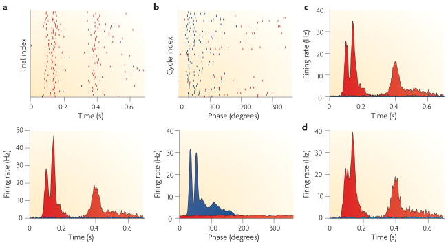
A model cell was embedded in a network producing a delta oscillation. A stimulus lasting 0.7 seconds was presented 1,000 times, with a random interval between presentations. As a first approximation it was assumed that the stimulus and the oscillation elicited independent precise spike patterns. a| The response of the neuron aligned with the stimulus onset. b| The response aligned with the oscillation cycle, where the x ordinate for each spike is its phase with respect to the oscillation. The top panel contains a rastergram across the first 50 stimulus presentations (the data in blue) and a rastergram across the first 50 oscillation cycles (the data in red). The bottom panel shows the corresponding spike-time histograms across all data, with the stimulus-related spikes in red and the oscillation-related spikes in blue. When they are aligned with the stimulus onset, the stimulus-induced spikes are precise and the oscillation-related spikes form a random background. When the data are aligned on the oscillation cycle the situation is reversed, with the stimulus-related spikes forming a random background. c,d. Under realistic circumstances, there will be interaction between the stimulus-related and the oscillation-related synaptic inputs. Two simple cases are illustrated using the stimulus-aligned spike-time histograms. c| The delta oscillation modulated the number of spikes that were elicited by the stimulus presentation, with the higher rates occurring at the beginning of the oscillation cycle. The precision (the width of the peaks) was not affected but the spike count across trials was much more variable. d| The delta oscillation shifted the times of the stimulus-elicited spikes depending on when they occurred in the oscillation cycle. This reduced the precision: the first two peaks seem to have merged. If stimulus-related information is to be coded in the precise spike times, the interaction illustrated in part c is innocuous but the one in part d is harmful.
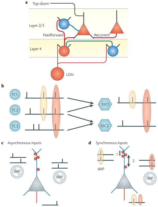
a| A simplified representation of the laminar structure of the feedforward pathway in cortical area V1. Thalamocortical (TC) cells project to spiny stellate cells (SSCs) in layer 4, which in turn project to layer 2/3 pyramidal cells. The layer 2/3 pyramidal cells receive feedforward input from layer 4, recurrent inputs from other pyramidal cells and top-down inputs from other cortical areas (such as V2). In both layer 4 and layer 2/3 there is feedforward inhibitory input. The inhibitory cells and their projections are shown in blue, whereas the excitatory cells and their projections are shown in red. b| TC cells project to SCCs in layer 4 of the sensory cortex. Experimental recordings of TC neurons indicate the presence of spike patterns,, which suggests that there are synchronous spike volleys at the population level. The spike volleys could be synchronous to a few SSCs (yellow highlight) or they could be synchronous across inputs to a large group of SSCs (red highlight). Synapses made by TC cells are more effective than intracortical synapses, but there are fewer of them. Nevertheless, because of synchronous spikes the TC cells as a group are effective. At the cortical level, this leads to synchronous output spikes across the SSC population when the synchrony extends across many TC cells (red highlight), but not when it is limited to only a few TC cells (yellow highlight). c,d. Pyramidal cells in layer 2/3 (REF. 140) and layer 5 (REF. 141) of the cortex, and those in hippocampus,, display dendritic action potentials (dAPs) that move towards the soma where, in many cases, they lead to a precise and reliable output spike. Experiments in the hippocampus that used caged glutamate established the conditions under which dAP are generated. c| dAP were not obtained when a pyramidal cell was stimulated by asynchronous spike trains. Target synapses are depicted as red circles. d| dAP were obtained when the input spike trains were synchronous and the synapses they activated were close together (clustered) on the dendrite (arrow 1; synaptic distance less than 20 μm); they were not obtained when the synapses were further apart (arrow 2; synaptic distance more than 20 μm). LGN, lateral geniculate nucleus.
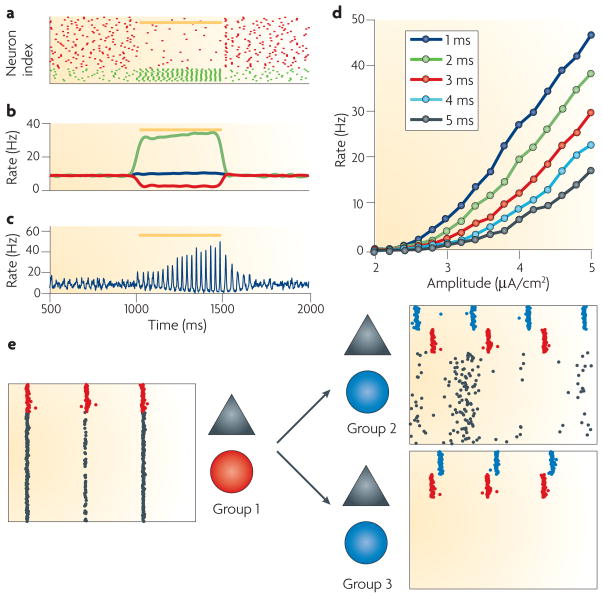
a –c. Synchrony by competition. A network model with Hodgkin–Huxley-type neurons was used for the simulations. a| In an inhibitory network of 1,000 neurons, 250 neurons (represented by the green dots) are transiently activated by a 500-ms depolarizing current pulse (represented by the yellow bar). The remaining 750 neurons (represented by the red dots) are not stimulated. The current pulse represents the effect of a top-down excitatory projection that has been hypothesized to mediate the effects of selective attention. b| The firing rate of the activated neurons increases (green line) but the mean stays approximately constant (blue line) because the non-activated neurons are suppressed (red line). c| The network as a whole synchronizes, as indicated by the sharper and higher peaks in the graph. d| The transformation of synaptic inputs into an output spike train is often characterized quantitatively as the firing rate (f) that is obtained in response to the injection of a current step as a function of the amplitude (I) of the step (the f–I characteristic). A gain change of the f–I means that, for the same value of I, a different firing rate is obtained (expressed as a gain factor (g) times the old firing rate (f)). The gain change is multiplicative when g is independent of the value of I. Changes in the synchrony (precision) of inhibitory inputs, such as those that are generated in the interneuron network in a, change the gain of postsynaptic neurons in an approximately multiplicative way. Decreasing jitter increases the firing rate. The value of the jitter for each curve, expressed in milliseconds, is shown in the key. The data were obtained from simulations of a single-compartment model. e| An example of selective communication using phase relationships. There were 3 pools of neurons, each comprising 200 pyramidal cells (represented by the black triangles) and 50 interneurons (represented by the blue and red circles). The group 1 neurons projected to the group 2 and 3 neurons. The rastergrams are colour-coded according to the colour of the symbol for each cell group. The interneurons in each group were synchronized but had different phases. Group 1 interneurons (represented by the red dots) lagged behind those in group 2 (represented by the blue dots in the right-hand upper panel) but led those in group 3 (represented by the blue dots in the right-hand lower panel). As a result, when an excitatory volley from group 1 (represented by the black dots in the left-hand panel) arrived in group 2, the inhibition had already partially decayed and the neurons responded (represented by the black dots in the right-hand upper panel). Conversely, for group 3 the excitatory volley arrived at the time with the highest inhibition, and no spikes were produced. The spikes of the interneuron network in group 1 (red dots) are repeated in the rastergrams for groups 2 and 3 to provide a reference time. Simulation data were obtained from a network model similar to one used previously to study attentional modulation in cortical area V4. Parts a and c reproduced, with permission, from REF. © (2004) MIT Press. Part d reproduced, with permission, from REF. © (2004) Elsevier Science.
References
-
- Mainen Z, Sejnowski T. Reliability of spike timing in neocortical neurons. Science. 1995;268:1503–1506. - PubMed
-
- Liu RC, Tzonev S, Rebrik S, Miller KD. Variability and information in a neural code of the cat lateral geniculate nucleus. J Neurophysiol. 2001;86:2789–2806. - PubMed
-
- Butts DA, et al. Temporal precision in the neural code and the timescales of natural vision. Nature. 2007;449:92–95. - PubMed
Publication types
MeSH terms
Grants and funding
LinkOut - more resources
Full Text Sources
