Quantifying hepatic shear modulus in vivo using acoustic radiation force

Abstract

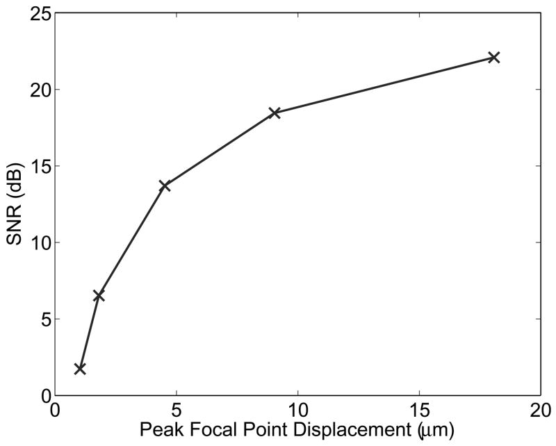
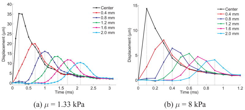
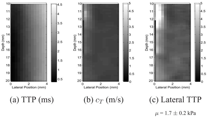
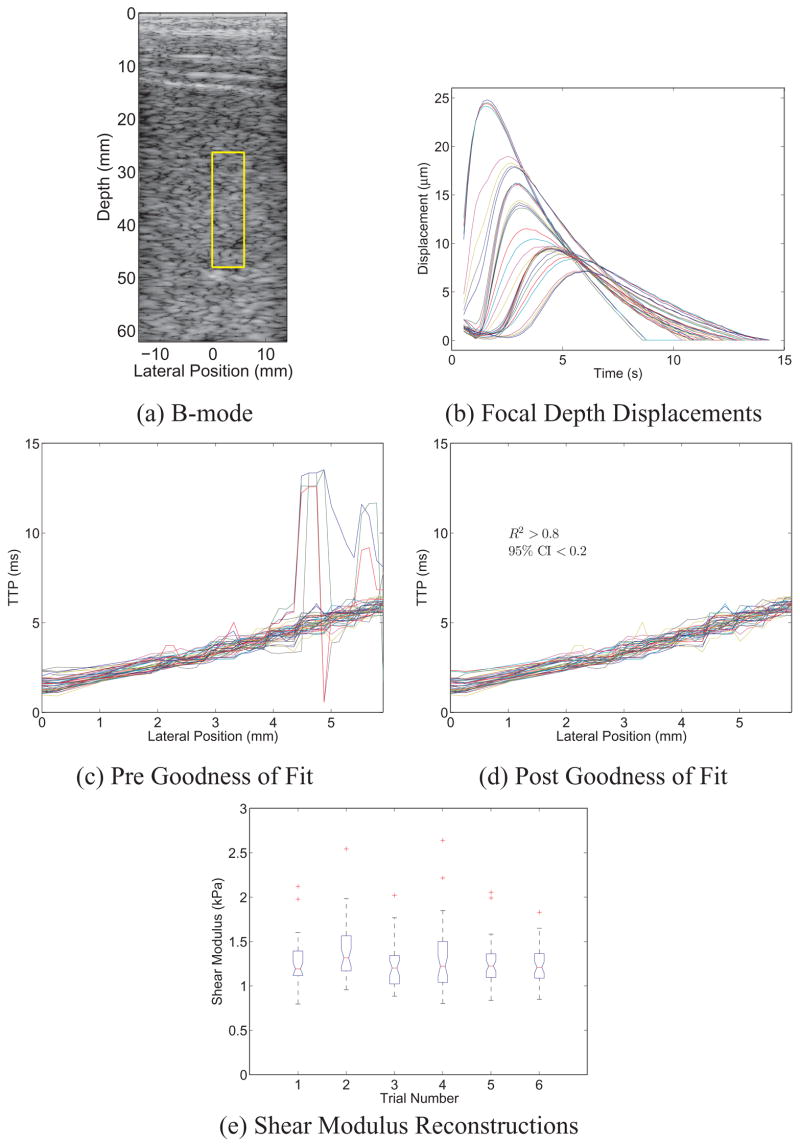
The speed at which shear waves propagate in tissue can be used to quantify the shear modulus of the tissue. As many groups have shown, shear waves can be generated within tissues using focused, impulsive, acoustic radiation force excitations, and the resulting displacement response can be ultrasonically tracked through time. The goals of the work herein are twofold: (i) to develop and validate an algorithm to quantify shear wave speed from radiation force-induced, ultrasonically-detected displacement data that is robust in the presence of poor displacement signal-to-noise ratio and (ii) to apply this algorithm to in vivo datasets acquired in human volunteers to demonstrate the clinical feasibility of using this method to quantify the shear modulus of liver tissue in longitudinal studies. The ultimate clinical application of this work is noninvasive quantification of liver stiffness in the setting of fibrosis and steatosis. In the proposed algorithm, time-to-peak displacement data in response to impulsive acoustic radiation force outside the region of excitation are used to characterize the shear wave speed of a material, which is used to reconstruct the material's shear modulus. The algorithm is developed and validated using finite element method simulations. By using this algorithm on simulated displacement fields, reconstructions for materials with shear moduli (mu) ranging from 1.3-5 kPa are accurate to within 0.3 kPa, whereas stiffer shear moduli ranging from 10-16 kPa are accurate to within 1.0 kPa. Ultrasonically tracking the displacement data, which introduces jitter in the displacement estimates, does not impede the use of this algorithm to reconstruct accurate shear moduli. By using in vivo data acquired intercostally in 20 volunteers with body mass indices ranging from normal to obese, liver shear moduli have been reconstructed between 0.9 and 3.0 kPa, with an average precision of +/-0.4 kPa. These reconstructed liver moduli are consistent with those reported in the literature (mu = 0.75-2.5 kPa) with a similar precision (+/-0.3 kPa). Repeated intercostal liver shear modulus reconstructions were performed on nine different days in two volunteers over a 105-day period, yielding an average shear modulus of 1.9 +/- 0.50 kPa (1.3-2.5 kPa) in the first volunteer and 1.8 +/- 0.4 kPa (1.1-3.0 kPa) in the second volunteer. The simulation and in vivo data to date demonstrate that this method is capable of generating accurate and repeatable liver stiffness measurements and appears promising as a clinical tool for quantifying liver stiffness.

Figure 1

Times to peak displacement along the imaging plane in FEM data from simulated elastic materials with shear moduli of 2.8, 7.7, and 16.0 kPa. The horizontal dashed lines represent the DOF over which shear wave reconstructions were performed on data throughout this manuscript. The colorbar represents TTP displacement in milliseconds, and a lateral position of 0 corresponds to the center of the ROE.

Figure 2

Peak displacement SNR over a 6 mm lateral range adjacent to the ROE for varying peak displacement magnitudes at the focal point. The SNR was computed as the mean/standard deviation of peak displacement estimates over the 6 mm lateral range for 20 independent, simulated speckle realizations from FEM displacement data.

Figure 3

Simulated displacement through time profiles, without ultrasonic tracking, at lateral positions offset from the excitation location for elastic media with shear moduli of (a) 1.33 kPa and (b) 8 kPa. Notice that the curve appears more finely sampled in the more compliant medium (1.33 kPa) due to its slower propagation speed and the fixed 10 kHz temporal sampling (simulating a fixed PRF in the experimental system). The vertical dotted lines indicate the TTP values that would be estimated from this data, though experimentally the data would be upsampled using a low-pass interpolation from the acquired PRF to 50 kHz. Notice that the two plots are on different time scales.

Figure 4

(a) Time to peak (TTP) displacement data at the focal depth (20 mm) as a function of lateral position in simulation data for elastic materials with shear moduli of 1.33 and 2.83 kPa. The inverse slopes of these lines represent the shear wave speeds in these materials. (b) Reconstructed shear moduli over depths from 16–20 mm (focal depth) using the Lateral TTP algorithm on the simulated datasets for 1.33 (x) and 2.83 (o) kPa shear moduli. The non-tracked FEM data are represented by the red (x) and blue (o) lines, with the mean ± one standard deviation shear modulus estimates over the range of depths represented in each colored text box. The corresponding tracked data, using 20 independent speckle realizations, is shown in the black lines (mean ± one standard deviation), for the 1.33 (x) and 2.82 (o) kPa media, again with the text boxes representing the mean ± one standard deviation shear modulus estimates over the range of depths.

Figure 5

Reconstructed shear moduli using the Lateral TTP algorithm on ultrasonically-tracked and raw FEM displacement data for shear moduli ranging from 1.33–16 kPa. The errors bars in the raw FEM data represent the variation in the reconstructed moduli over the DOF, while the error bars in the tracked FEM data represent the variation over 20 independent speckle realizations at the focal depth (20 mm).

Figure 6

Shear modulus reconstruction in a elastic gelatin phantom. (a) The TTP displacement is estimated over the ROI. (b) Locally estimated shear wave speeds by taking the inverse of the slope of the TTP at each pixel as a function of lateral position for each depth, with a sliding window for the linear regression. (c) Localized shear modulus image obtained using the Lateral-TTP algorithm (μ = 1.7 ± 0.2 kPa).

Figure 7

(a) B-mode image from a human volunteer, with the ROI used for shear wave speed characterization by the Lateral TTP algorithm outlined by the yellow box. The radiation force excitation was focused at 37.5 mm at a lateral position of 0. (b) Motion-filtered displacement through time data at the focal depth, representing one of many depth increments analyzed over the DOF of the excitation beam. The different color lines represent the different lateral positions in the ROI, with curves peaking later in time being more laterally offset from the ROE. (c & d) Times to peak displacement as a function of lateral position for each of the depth increments analyzed over the DOF, pre and post application of the goodness of fit metrics (R² > 0.8, 95% CI < 0.2). (e) Box plots of the reconstructed shear moduli from the six independent data acquisitions in this volunteer. The box plots represents the distribution of shear moduli over the DOF, with each box representing the interquartile range (IQR) of reconstructed moduli with the horizontal line representing the median value. The whiskers represent ±1.5 IQR, with outliers indicated by a ‘+’ symbol.

Figure 8

(a) In vivo liver shear moduli estimates in twenty human volunteers using an intercostal imaging approach between the ninth and tenth ribs. (b) Comparison of reconstructed in vivo liver shear moduli in two human volunteers over a four month period. Six measurements were performed intercostally on each day in each volunteer between the ninth and tenth ribs. In both (a) and (b), the reconstructed shear moduli represent the mean and standard deviation over six independent measurements, where values that didn’t meet the goodness of fit parameters (R² > 0.8, 95% CI < 0.2) or were greater than one standard deviation from the mean for a given measurement were excluded from the analysis. (c) Mean reconstructed shear moduli in the 20 volunteers as a function of their BMI. The left vertical dashed line represents the distinction between normal and overweight volunteers, while the right vertical dashed line represents the distinction between overweight and obese volunteers.

References

1. Bedossa P, Dargere D, Paradis V. Sampling variability of liver fibrosis in chronic hepatitis c. Hepatology. 2003;38(1):1449–1457. - PubMed
1. Bercoff J, Tanter M, Fink M. Supersonic shear imaging: A new technique for soft tissue elasticity mapping. IEEE Trans Ultrason, Ferroelec, Freq Contr. 2004;51(4):396–409. - PubMed
1. Christensen D. Ultrasonic Bioinstrumentation. New York: John Wiley & Sons; 1988.
1. Dahl J, Palmeri M, Agrawal V, Nightingale K, Trahey G. A parallel tracking method for acoustic radiation force impulse imaging. IEEE Trans Ultrason, Ferroelec, Freq Contr. 2007;54(2):301–312. - PMC - PubMed
1. Foucher J, Chanteloup E, Vergniol J, Castera L, LeBail B, Adhoute X, Bertet J, Couzigou P, deLedinghen V. Diagnosis of cirrhosis by transient elastography (fibroscan): a prospective study. Gut. 2006;55(1):403–408. - PMC - PubMed
Publication types