Incorporating the effects of transcytolemmal water exchange in a reference region model for DCE-MRI analysis: theory, simulations, and experimental results

Abstract

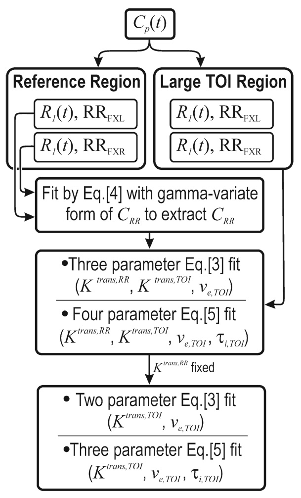
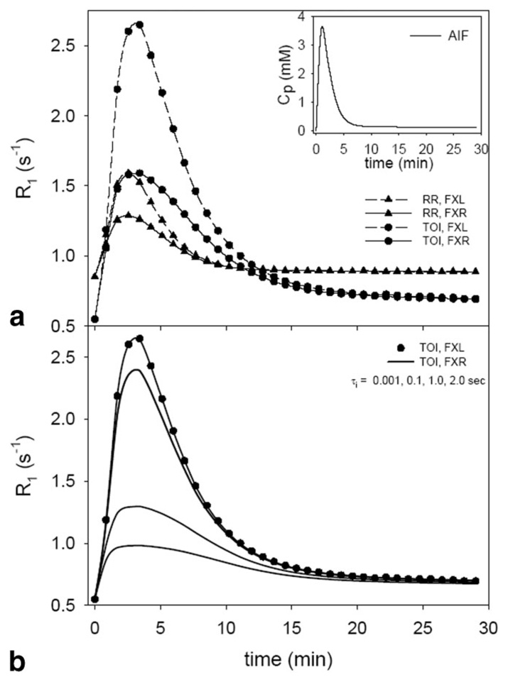
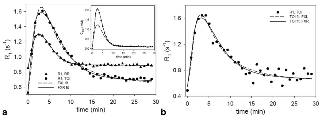
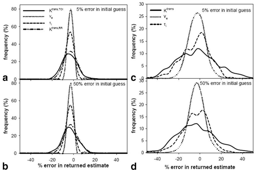
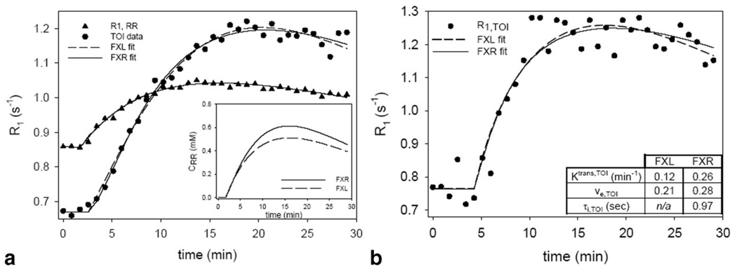
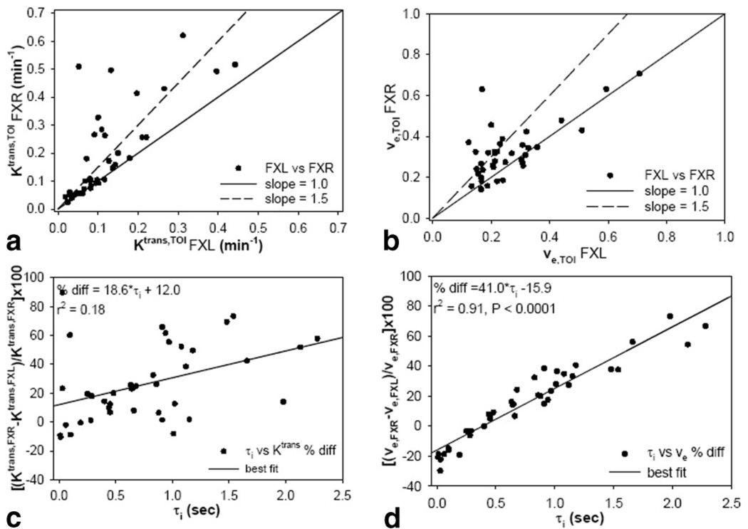
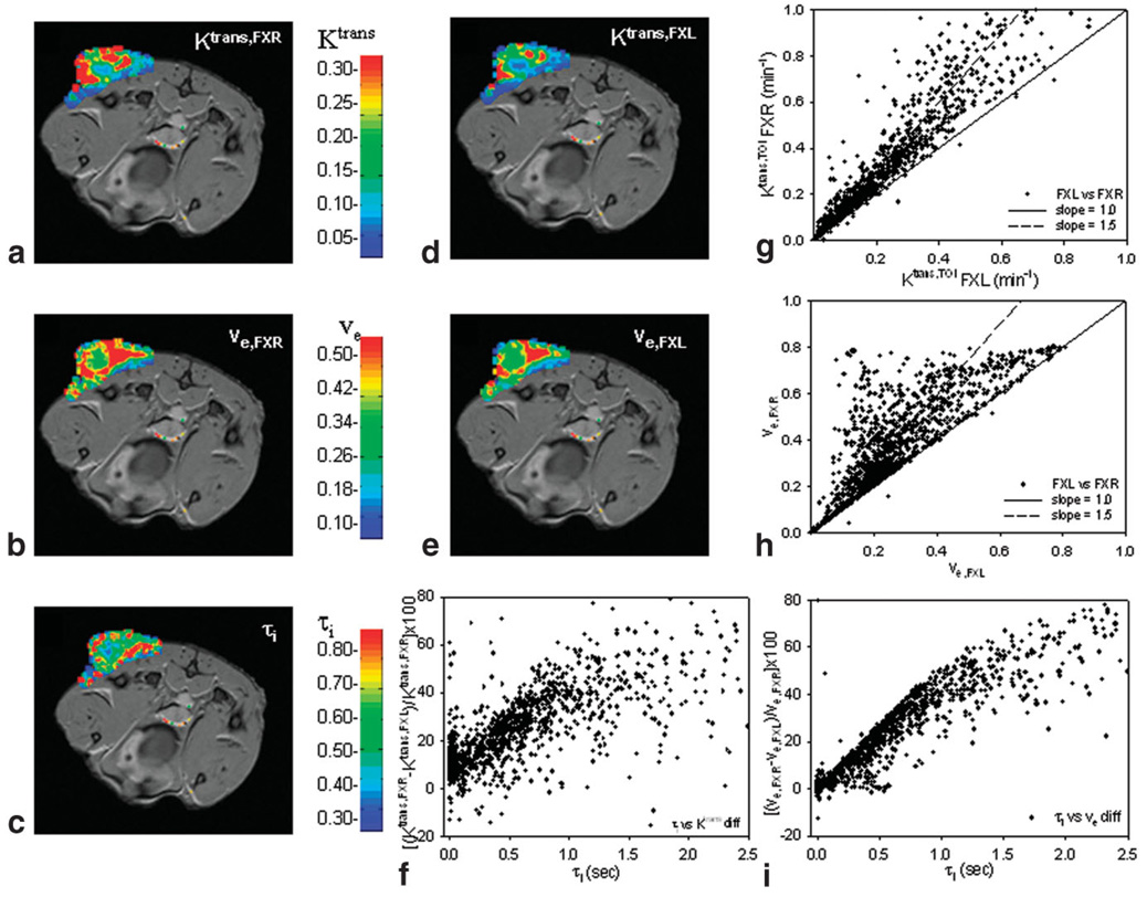
Models have been developed for the analysis of dynamic contrast-enhanced MRI (DCE-MRI) data that do not require direct measurements of the arterial input function; such methods are referred to as reference region models. These models typically return estimates of the volume transfer constant (K(trans)) and the extravascular extracellular volume fraction (v(e)). To date such models have assumed a linear relationship between the measured R(1) ( identical with 1/T(1)) and the concentration of contrast agent, a transformation referred to as the fast exchange limit, but this assumption is not valid for all concentrations of an agent. A theory for DCE-MRI reference region models which accounts for water exchange is presented, evaluated in simulations, and applied in tumor-bearing mice. Using reasonable parameter values, simulations show that the assumption of fast exchange can underestimate K(trans) and v(e) by up to 82% and 46%, respectively. By analyzing a large region of interest and a single voxel the new model can return parameters within approximately +/-10% and +/-25%, respectively, of their true values. Analysis of experimental data shows that the new approach returns K(trans) and v(e) values that are up to 90% and 73%, respectively, greater than conventional fast exchange analyses.

FIG. 1

The flow chart indicates how the simulations were performed. First an arterial input function was assumed and used to create R₁ time courses using both the FXL and FXR formalism. The R₁ time course from a large region of interest within (simulated) muscle tissue is then used to extract a C_RR time course. A three-parameter FXL-RR and a four-parameter FXR-RR fit are then performed to determine a value for K^trans,RR, which is then assigned so that subsequent two-parameter (K^trans and v_e) FXL-RR fit and three-parameter (K^trans, v_e, and τ_i) FXR-RR fits can be performed on a voxel-by-voxel basis.

FIG. 2

a: The AIF (inset) used to drive the simulations and the results of R₁ time courses for the reference region (RR) and tissue of interest (TOI). One set of parameter values was used to make both RR curves and another set were used to make both TOI curves. The differences in R₁ time courses as predicted by the FXL and FXR models are evident. b: Highlights that the FXR curve shape converges to the FXL curve shape as the value of τ_i is reduced.

FIG. 3

The results of fitting simulated data to the FXL-RR and FXR-RR models. a: The three-parameter FXL-RR fits and the four-parameter FXR-RR fits to high SNR data simulating a large region of interest. It is evident that the FXL models display a systematic deviation from the data by first overshooting the peak of the data and then oscillating below and above the data. b: The two-parameter FXL-RR and the three-parameter FXR-RR fits. Again, a systematic deviation from the data is evident. The parameter estimates returned by each model are presented in the table.

FIG. 4

a,b: The error in the returned estimate when the initial guesses are within 5% and 50%, respectively, of the correct value when the four-parameter FXR-RR model is used. As long as the initial guess is within 50% of the value, the model seems to be stable to noise levels seen in a large region of interest that would be used in the three-parameter fit. c,d: The error in the returned estimate when the initial guesses are within 5% and 50%, respectively, of the correct value when the three-parameter FXR-RR model is used. The three-parameter fit is used for single voxel analysis and the SNR is significantly reduced when compared to a large region of interest and this translates into less certainty about the returned value.

FIG. 5

The results of fitting experimental data to the FXL-RR and FXR-RR models. a: The three-parameter FXL-RR fits and the four-parameter FXR-RR fits to high SNR data from a large region of interest. The systematic FXL error seen in the Fig. 3 simulations is also displayed here. b: The two-parameter FXL-RR and the three-parameter FXR-RR fits and the characteristic FXL mismatch is again evident. The parameter values returned by these fits are presented in the inset in b.

FIG. 6

a,b: Scatterplots of K^trans,TOI and v_e,TOI, respectively, as returned by the FXL-RR and FXR-RR models for all 40 voxels randomly selected from each mouse tumor (five voxels per mouse). It is evident that the FXL model consistently reports parameter values below that returned by the FXR model. c,d: Scatterplot of the percent difference between K^trans and v_e, respectively, as a function of τ_i value. As τ_i increases there is a trend for the two models to have a great disparity; this trend is significant in the v_e plot (d) but not in the K^trans plot (c).

FIG. 7

The results of parametric maps by both models of a representative mouse. The K^trans (a) and v_e FXR (b) maps show increased number of red voxels when compared to the corresponding FXL maps (d,e) and this trend is made quantitative in the scatter plots (g,h). f,i: The percent difference between the two models as presented in Fig. 6c,d; the same trend is evident as in Fig. 6 but the linearity of the relationship tends to diminish once τ_i moves above 1.0 sec in this animal. The scatterplots indicate all (approximately) 2000 voxels across all slices of this tumor. Also, the color maps are superimposed on the tenth postcontrast image and represent the SNR that is used to construct these parametric maps.

References

1. Tofts PS, Brix G, Buckley DL, Evelhoch JL, Henderson E, Knopp MV, Larsson HBW, Lee T-Y, Mayr NA, Parker GJM, Port RE, Taylor J, Weisskoff RM. Estimating kinetic parameters from dynamic contrast-enhanced T1-weighted MRI of a diffusible tracer: standardized quantities and symbols. J Magn Reson Imaging. 1999;10:223–232. - PubMed
1. Yankeelov TE, Gore JC. Dynamic contrast enhanced magnetic resonance imaging in oncology. Curr Med Imaging Rev. 2007;3:91–107. - PMC - PubMed
1. Lankester KJ, Taylor NJ, Stirling JJ, Boxall J, D’Arcy JA, Leach MO, Rustin GJ, Padhani AR. Effects of platinum/taxane based chemotherapy on acute perfusion in human pelvic tumours measured by dynamic MRI. Br J Cancer. 2005;93:979–985. - PMC - PubMed
1. Li KL, Wilmes LJ, Henry RG, Pallavicini MG, Park JW, Hu-Lowe DD, McShane TM, Shalinsky DR, Fu YJ, Brasch RC, Hylton NM. Heterogeneity in the angiogenic response of a BT474 human breast cancer to a novel vascular endothelial growth factor-receptor tyrosine kinase inhibitor: assessment by voxel analysis of dynamic contrast-enhanced MRI. J Magn Reson Imaging. 2005;22:511–519. - PubMed
1. Wang B, Gao ZQ, Yan X. Correlative study of angiogenesis and dynamic contrast-enhanced magnetic resonance imaging features of hepatocellular carcinoma. Acta Radiol. 2005;46:353–358. - PubMed
Publication types