The peri-saccadic perception of objects and space

Abstract

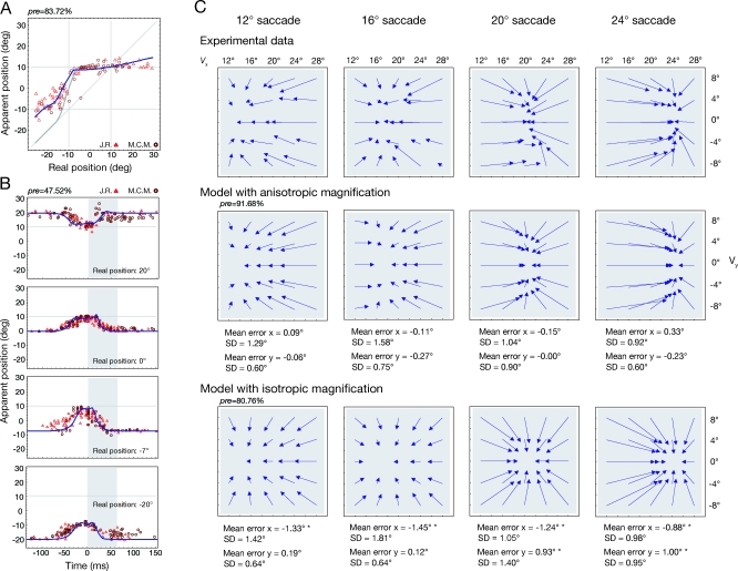
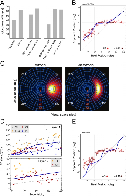
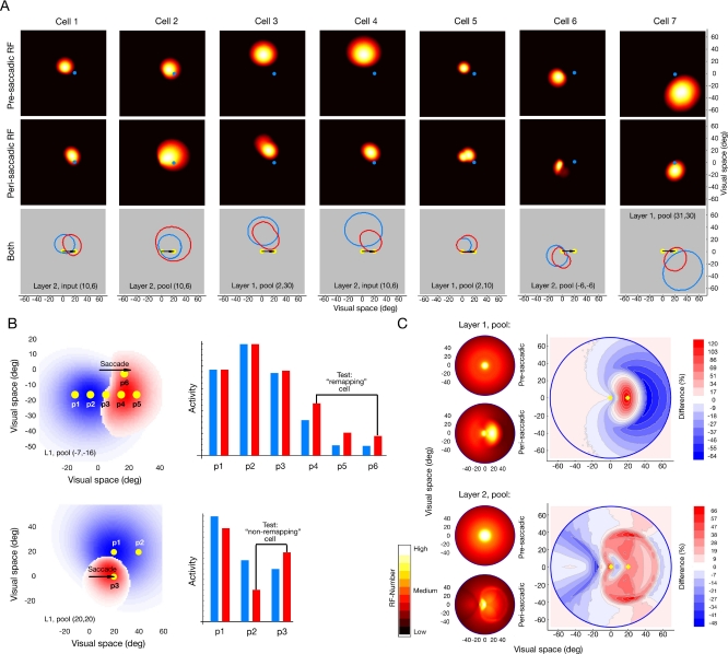
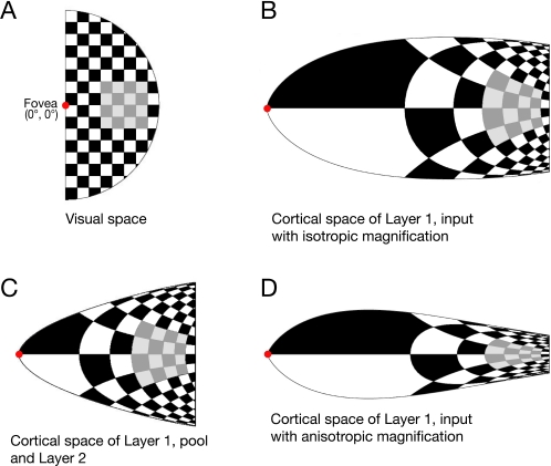
Eye movements affect object localization and object recognition. Around saccade onset, briefly flashed stimuli appear compressed towards the saccade target, receptive fields dynamically change position, and the recognition of objects near the saccade target is improved. These effects have been attributed to different mechanisms. We provide a unifying account of peri-saccadic perception explaining all three phenomena by a quantitative computational approach simulating cortical cell responses on the population level. Contrary to the common view of spatial attention as a spotlight, our model suggests that oculomotor feedback alters the receptive field structure in multiple visual areas at an intermediate level of the cortical hierarchy to dynamically recruit cells for processing a relevant part of the visual field. The compression of visual space occurs at the expense of this locally enhanced processing capacity.

Figure 1. Computational Model for the Oculomotor Modulation of Visual Processing

(A) Hierarchical view of visual processing where each cell implements a specific feature detector with a localized receptive field. Each layer consists of three stages (input, gain and pool). The oculomotor system feeds the encoded saccade target position back to multiple layers and increases the gain of the cells prior to spatial pooling. (B) Illustration of the mapping from visual space to cortical space. (C) Detailed view of computations within a single layer. We illustrate the effect on the population response exerted by a peri-saccadically flashed dot at position (16°, 8°) while executing a 24° saccade. The activity distributions in the model are shown in cortical space. The depicted area of cortical space refers to the gray surface highlighted in the visual space. The spatial distortion due to cortical magnification is illustrated by the projection of the grid in the visual space into the cortical space. Using functions of receptive field size, cortical magnification and gaze position, we first determine the cortical population response in the input stage evoked by the flashed dot. The feedback signal determines the gain factor according to its activity profile. The gain modulated population response is distorted towards the saccade target. This population is then spatially pooled to obtain increasing spatial invariance. The perceived position of the stimulus is decoded from the activity in the neural ensemble. (D) Population responses along the horizontal meridian in layer 1, input and layer 1, gain from a flashed dot at position (10°, 0°) before a 20° saccade. Long before saccade onset (t < −150 ms) no oculomotor feedback has been built up and the population responses in layer 1, input and layer 1, gain are identical. The decoding of the stimulus position from the population response leads to the true position. At t = −40 ms oculomotor feedback is sufficiently strong to distort the population response so that the decoded value is already shifted towards the saccade target. As the occurrence of the flash gets closer to saccade onset, the feedback signal, and thus the gain, increases further and the estimated perceived position is close to the saccade target. However, a further increase of the gain (e.g., flash occurrence at t = −20 ms) does not lead to a larger mislocalization.

Figure 2. Peri-Saccadic Compression in the Model

(A) Spatial range of compression. The data shows the apparent versus real position of flashed bars in the critical phase from −25 to 0 ms before a 20° saccade for two human subjects (data from Morrone et al. [9]). Estimated stimulus location by the model using L₁ and L₂ (blue) and only L₁ (gray). The area around the saccade target is compressed in L₁ whereas stimuli presented at large distances from the saccade target require another layer (L₂) with larger receptive field sizes. (B) The time course of compression. The data shows the apparent position of bars presented at four different locations as a function of time relative to saccade onset of two subjects (data from Morrone et al. [9]). The blue line represents the predicted mislocalization of the model. (C) The spatial pattern of compression. The data shows the absolute mislocalization with reference to the true position of a flashed dot randomly chosen from an array of 24 dots for four different saccade amplitudes (data replotted from Kaiser and Lappe [11], who plotted the mislocalization relative to a baseline). Vector origins indicate the veridical flash position and vector endpoints indicate the perceived position around saccade onset. The simulation results show the best fits of models with anisotropic or isotropic magnification. In contrast to the isotropic model, the anisotropic model on average does not significantly deviate from the data (section “Computation of mean errors”). Significant deviations (p < 0.05) are indicated by * (two-sided one-sample t-test, α = 0.05, df = 23).

Figure 3. Predicted Source and Shape of Oculomotor Feedback, and Predicted Target Area of Compression

(A) Goodness of fit (pre) for the time course and spatial range of compression with respect to typical properties of cells in oculomotor areas. Unclipped activity and open movement fields lead to a drop in the goodness of fit. A time course which resembles the firing pattern of burst cells is consistent with the data, whereas build-up like activity with a half maximum value around 46 ms prior to saccade requires a damped gain function in the target area to compensate the early distortion. (B) Effect of open movement fields on the localization of flashed bars in the critical phase from −25 to 0 ms before a 20° saccade. (C) Predicted shape of the feedback signal in visual space for a 20° saccade. The model with anisotropic magnification predicts a shape that is circumscribed for a particular eccentricity but spreads to different angles with constant eccentricity. For comparison, the model with isotropic magnification produces a round shape with a strong spread of the signal to a broader range of eccentricities. (D) Comparison of monkey receptive field sizes with the model prediction (Text S2). The line shows the required minimal receptive field size for each layer. Please note, due to the non-linear spatial pooling in the model, the receptive field values are upper bounds and not mean values. The dots indicate the maximal receptive field size for a particular eccentricity in the respective cortical area as reported in the literature. For the area to be consistent with the model the dots should be close to or exceed the constraint given by the model. Layer 1: The receptive field sizes in V4 are close to the minimal receptive field size of L₁. Receptive field sizes in MT and TEO are sufficiently large. Layer 2: Both TE and LIP are consistent with the prediction of the model for L₂. For larger eccentricities, receptive field sizes in LIP are below the lower limit obtained from the model. However, since the critical stimuli in the data (Figure 2A) which constrain the receptive field size in L₂ were all presented at an eccentricity of less than 20° (in the opposite hemifield than the one where the saccade target appeared) we should not exclude LIP. (E) Effect of small receptive field sizes in L₁ and L₂ (dashed lines in [D]) on the localization of flashed bars in the critical phase from −25 to 0 ms before a 20° saccade.

Figure 4. Predicted Receptive Field Dynamics and Capacity Increase

(A) Pre- and peri-saccadic receptive fields of seven representative model cells for a rightward saccade of 20° as determined by a half-maximum threshold. Layer of origin and the location of the receptive field centers are given in the lower plots. The yellow and blue dots indicate fixation and saccade target position whereas the arrow shows the saccade vector. (B) Peri-saccadic receptive field changes of two cells. The blue color indicates the pre-saccadic activity profile and the red color the peri-saccadic one. If the peri-saccadic response is larger, it is shown on top of the pre-saccadic one. The yellow dots indicate probe positions and the response to each probe is plotted to the right. The cell in L_1,pool with a pre-saccadic receptive field center at (−7°,−16°) remaps with the saccade vector, comparable to electrophysiological observations [7], since the peri-saccadic change in response is maximal around p4. The receptive field does not shift to the saccade target since the response at p6 is lower than the one at p4 and about the same as at p5. The cell in L_1,pool with a pre-saccadic receptive field center at (20°,20°) shows by no means remapping. The peri-saccadic response at p3 is higher than the one at p2. (C) The pre- and peri-saccadic processing capacity as estimated by the number of neurons participating in the processing of each part of the visual field. For each position (squared area of 1°) in the visual field we counted the number of selective cells as determined by the mapped receptive field. Due to cortical magnification the pre-saccadic case shows a high capacity in the center. In the peri-saccadic case the model predicts a strong increase around the saccade target. The relative change in processing capacity reveals the areas of increase and decrease in the visual field. In L_1,pool the capacity increases around the saccade target and in L_2,pool we observe a rough hemispheric effect. The yellow dots indicate the fixation and the saccade target.

Figure 5. Gain of a Neuron i with Respect to the Feedback Strength for an Input = 0.1

The gain is equal to 1, if no feedback signal is present. An increase of the feedback signal enhances the gain of a neuron. (A) Instantaneous gain function. (B) Damped gain function.

Figure 6. Visual Hemifield and the Respective Side View of the Different Cortical Model Surface from the Fovea up to 32° Eccentricity

The center of the visual field, i.e., the fovea, is indicated by the red dot. Each checkerboard element is 4° by 4° in visual space. The gray shaded part indicates the area where the dots in the experiment of Kaiser and Lappe [11] were presented. (A) Visual space. (B) Layer 1, input with isotropic magnification (M_p = M_e). (C) Layer 1, pool and Layer 2. (D) Layer 1, input with anisotropic magnification (M_p > M_e).

Figure 7. Simulated Saccade

(A) Velocity profile a of simulated 20° saccade. (B) Position of the eye relative to the FP at 0°.

References

1. Hoffman JE, Subramaniam B. The role of visual attention in saccadic eye movements. Percept Psychophys. 1995;57:787–795. - PubMed
1. Deubel H, Schneider WX. Saccade target selection and object recognition: Evidence for a common attentional mechanism. Vision Res. 1996;36:1827–1837. - PubMed
1. Tolias AS, Moore T, Smirnakis SM, Tehovnik EJ, Siapas AG, Schiller PH. Eye movements modulate visual receptive fields of V4 neurons. Neuron. 2001;29:757–767. - PubMed
1. Duhamel JR, Colby CL, Goldberg ME. The updating of the representation of visual space in parietal cortex by intended eye movements. Science. 1992;25:90–92. - PubMed
1. Walker MF, Fitzgibbon EJ, Goldberg ME. Neurons in the monkey superior colliculus predict the visual result of impending saccadic eye movements. J Neurophysiol. 1995;73:1988–2003. - PubMed
Publication types