Spatial heterogeneity of cortical receptive fields and its impact on multisensory interactions

Abstract

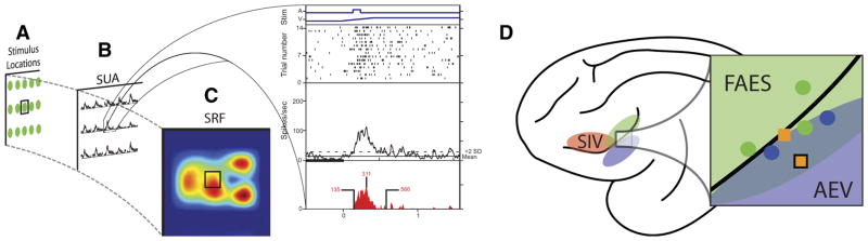
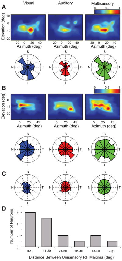
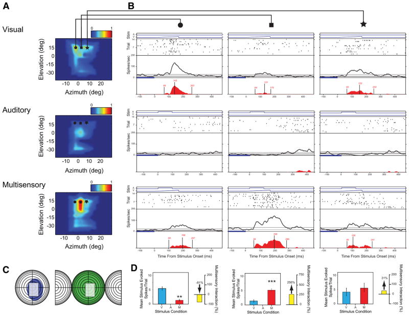
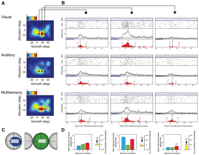
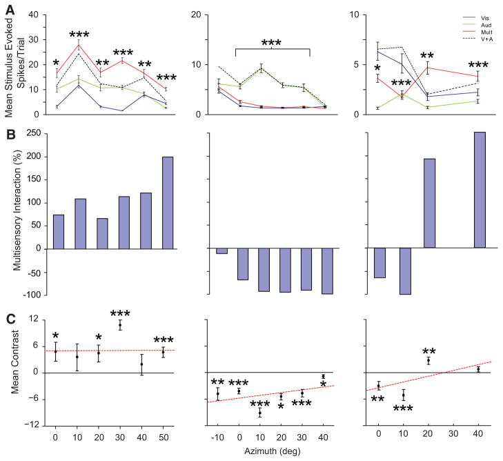
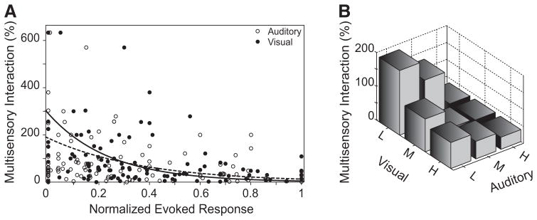
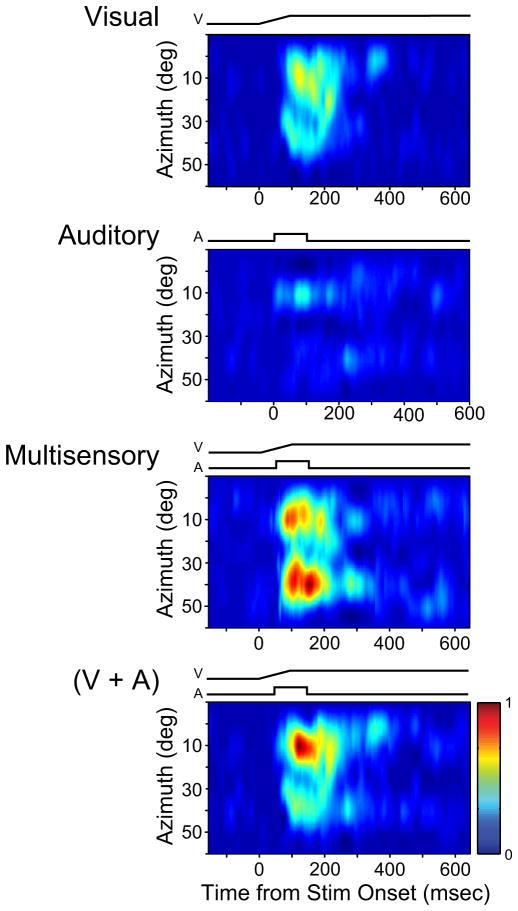
Investigations of multisensory processing at the level of the single neuron have illustrated the importance of the spatial and temporal relationship of the paired stimuli and their relative effectiveness in determining the product of the resultant interaction. Although these principles provide a good first-order description of the interactive process, they were derived by treating space, time, and effectiveness as independent factors. In the anterior ectosylvian sulcus (AES) of the cat, previous work hinted that the spatial receptive field (SRF) architecture of multisensory neurons might play an important role in multisensory processing due to differences in the vigor of responses to identical stimuli placed at different locations within the SRF. In this study the impact of SRF architecture on cortical multisensory processing was investigated using semichronic single-unit electrophysiological experiments targeting a multisensory domain of the cat AES. The visual and auditory SRFs of AES multisensory neurons exhibited striking response heterogeneity, with SRF architecture appearing to play a major role in the multisensory interactions. The deterministic role of SRF architecture was tightly coupled to the manner in which stimulus location modulated the responsiveness of the neuron. Thus multisensory stimulus combinations at weakly effective locations within the SRF resulted in large (often superadditive) response enhancements, whereas combinations at more effective spatial locations resulted in smaller (additive/subadditive) interactions. These results provide important insights into the spatial organization and processing capabilities of cortical multisensory neurons, features that may provide important clues as to the functional roles played by this area in spatially directed perceptual processes.

Fig. 1

Construction of spatial receptive field (SRF) plots and location of recorded neurons. A: an example array of spatial locations (green dots) in which visual, auditory, and paired visual–auditory stimuli are presented to a multisensory neuron. B: the single-unit activity (SUA) at each of the tested locations is represented as stimulus-evoked spike density functions. The expansion box shows the raw data for a multisensory response at a single location and is composed of 4 panels. The top panel shows the visual (V: movement depicted by ramp) and auditory (A: square wave) stimulus onset and offset times. The 2nd panel shows a raster plot of the neuronal response, with each dot representing an action potential and each row representing a single trial. The 3rd panel shows a collapsed spike density function, with the dotted line representing the response level 2SDs above baseline (i.e., the response criterion). The bottom panel shows only the statistically defined evoked response (red shading) and illustrates various aspects of the temporal dynamics (onset, peak, and offset) of the evoked response. C: the evoked response at each location is then normalized to the greatest elicited response across conditions, with the warmth of the color representing the magnitude of the response. D: shown on the schematic view of lateral surface of the cat brain is the location of electrode penetrations through anterior ectosylvian sulcus (AES) cortex for one animal. Colored shading highlights the 3 unisensory subdivisions of the AES cortex: 4th somatosensory cortex (SIV, red), auditory field AES (FAES, green), and anterior ectosylvian visual area (AEV, blue). The circles represent penetrations in which only unisensory units were isolated, with the color representing the effective modality (visual: blue; auditory: green). Squares represent penetrations in which multisensory neurons (visual–auditory) were isolated and recorded; the black outlined square represents the location of the penetration in which the unit in Fig. 4 was recorded. Note that multisensory units were isolated on penetrations located on the border between FAES and AEV. Due to the complex geometry of the AES, only penetrations in which the approach angle was equivalent are shown in this figure.

Fig. 2

Examples of response heterogeneity in the SRFs of cortical multisensory neurons. A: the visual, auditory, and multisensory SRFs for the region of receptive field overlap in an AES neuron (SRFs constructed as detailed in Fig. 1). Each of the 3 representations has been normalized to the greatest evoked response, with the pseudocolor plots showing the relative activity scaled to this maxima. Below the SRFs are polar plots in which the center of the plot is the geometric center of the tested area of overlap. The magnitude of each wedge is proportional to the evoked response in that region of the receptive field, normalized across conditions (N, nasal; T, temporal; S, superior; I, inferior). B: an example of SRF and polar plots for a second AES multisensory neuron. Note in this example the substantial disparity between the visual and auditory SRFs. C: polar plot representations (grand mean) for the population of AES multisensory neurons. D: the distribution of the population of AES neurons plotted as a function of the Cartesian distance separating the location of the maximal visual and auditory responses. Note that the majority of neurons have a relatively close correspondence (i.e., <20°).

Fig. 3

Multisensory interactions in AES neurons can differ widely as a function of the location of the paired stimuli. A: visual, auditory, and multisensory SRFs plotted using an identical convention to that described in Figs. 1 and 2. Symbols relate to the spatial locations of the stimulus pairings represented in B. B: rasters and spike density functions (see expansion box of Fig. 1B) show the details of this neuron’s responses to the visual stimulus alone (top row), auditory stimulus alone (middle row), and the combined visual–auditory stimulus (bottom row) presented at 3 different azimuthal locations (circle, square, and star on the receptive field plots in A show the stimulus locations; columns show the evoked responses at these 3 different locations). C: conventional representations of receptive fields for this neuron, in which the shaded areas (blue: visual; green: auditory) depict the classically defined excitatory receptive field. In these plots, concentric circles represent 10°, with the split hemisphere on the auditory representation depicting caudal (behind the interaural plane) space. The gray area highlights the area of receptive field overlap in which the SRF plots were constructed. D: summary bar graphs illustrate the mean responses for the visual (blue), auditory (green), and multisensory (red) conditions, and the magnitude of the multisensory interaction (yellow) at each spatial location (**P < 0.01, ***P < 0.001). Note that despite the identical characteristics of the stimuli for each of these conditions (i.e., they vary only in spatial location), the magnitude of the visual response and the multisensory gain changes dramatically, shifting from response depression (circle column), to response enhancement (square column) to no interaction (star column).

Fig. 4

A second example of an AES neuron exhibiting substantial changes of response and multisensory interaction as a function of changes in stimulus location. Conventions are the same as in Fig. 3. This example differs from that shown in Fig. 3 by having a defined auditory response at each of the tested locations. Nonetheless, the same general pattern of results is seen. Here, whereas the pairing of effective visual and auditory stimuli resulted in no interaction (B, circle and square columns), pairings at a location in which the visual and auditory stimuli were less effective resulted in significant response enhancement (B, star column). (**P < 0.01).

Fig. 5

AES multisensory neurons can be divided into several operational categories based on how space influences their multisensory interactions. Shown in the 3 columns are data from 3 representative AES neurons. A: the mean visual (solid blue), auditory (solid green), multisensory (solid red), and predicted additive (i.e., V+A, dashed) responses for spatially coincident stimulus pairings at a number of azimuthal locations. B: bar graphs plot the sign and magnitude of the multisensory interaction as a function of spatial location. C: points and fitted lines show mean statistical contrast as a function of spatial location. Note that the neuron represented in the left column shows significant enhancements to all stimulus pairings and that these enhancements typically exceed the additive prediction (i.e., are superadditive). In contrast, the neuron in the middle column almost invariably exhibits response depressions, with the interactions being exclusively subadditive. The final example shows a more complex pattern of multisensory interactions, showing superadditive enhancements at some locations and subadditive interactions at other locations (*P < 0.05, **P < 0.01, ***P < 0.001).

Fig. 6

Changes in the multisensory interactive profile of AES neurons as a function of spatial location adhere to the principle of inverse effectiveness. A: a scatterplot of the magnitude of the multisensory interaction as a function of the normalized visual (black diamonds) or auditory (open circles) responses. The curves of best fit (modeled for both conditions with the exponential function [a × exp(bx)] for the visual (black dashed line, r² = 0.1238) and auditory (solid black line, r² = 0.2732) responses both show that as the magnitude of the evoked responses increase, the relative multisensory gain (i.e., interactive index) decreases. B: the bar graph divides normalized sensory evoked responses into low (L, 0–0.33), medium (M, 0.34–0.66), and high (H, 0.67–1.00) values across both sensory domains and shows that the largest multisensory interactions are found to pairings at locations where weak evoked stimulus responses are found (L visual, L auditory). In contrast, the smallest multisensory interactions are found at locations where maximal evoked stimulus responses (H visual, H auditory) are found in both domains. Note that as either of the unisensory responses increases independently there is a decrease in the size of the multisensory interaction.

Fig. 7

Temporal characteristics of stimulus-evoked responses change as a function of spatial location. Shown are spatiotemporal receptive field (STRF) plots for the visual, auditory, multisensory, and predicted addition (V+A) of the unisensory responses. Above each panel are stimulus traces that show stimulus onset and offset for each condition. The y-axis for all panels shows the azimuthal location of the stimulus (elevation was fixed at 0°). The x-axis for all panels shows the time relative to the earliest stimulus onset (t = 0). Note the difference in the temporal dynamics of the evoked responses (e.g., onset latency, duration, etc.) to the multisensory stimulus when compared with the unisensory STRFs or to the additive prediction.

References

1. Anastasio TJ, Patton PE. A two-stage unsupervised learning algorithm reproduces multisensory enhancement in a neural network model of the corticotectal system. J Neurosci. 2003;23:6713–6727. - PMC - PubMed
1. Anastasio TJ, Patton PE, Belkacem-Boussaid K. Using Bayes’ rule to model multisensory enhancement in the superior colliculus. Neural Comput. 2000;12:1165–1187. - PubMed
1. Avillac M, Deneve S, Olivier E, Pouget A, Duhamel JR. Reference frames for representing visual and tactile locations in parietal cortex. Nat Neurosci. 2005;8:941–949. - PubMed
1. Barraclough NE, Xiao D, Baker CI, Oram MW, Perrett DI. Integration of visual and auditory information by superior temporal sulcus neurons responsive to the sight of actions. J Cogn Neurosci. 2005;17:377–391. - PubMed
1. Beauchamp MS, Argall BD, Bodurka J, Duyn JH, Martin A. Unraveling multisensory integration: patchy organization within human STS multisensory cortex. Nat Neurosci. 2004;7:1190–1192. - PubMed
Publication types
LinkOut - more resources