SPACE: an algorithm to predict and quantify alternatively spliced isoforms using microarrays

Abstract

Exon and exon+junction microarrays are promising tools for studying alternative splicing. Current analytical tools applied to these arrays lack two relevant features: the ability to predict unknown spliced forms and the ability to quantify the concentration of known and unknown isoforms. SPACE is an algorithm that has been developed to (1) estimate the number of different transcripts expressed under several conditions, (2) predict the precursor mRNA splicing structure and (3) quantify the transcript concentrations including unknown forms. The results presented here show its robustness and accuracy for real and simulated data.

Figure 1

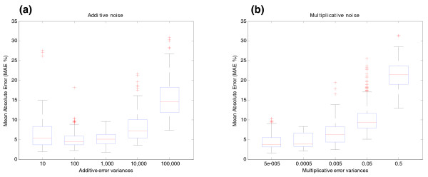
Influence of noise on the estimation of relative transcript concentrations of BIRC5 gene (synthetic data). BIRC5 gene structure is shown in Figure 6a and in Additional file 1 (Figure S4). (a) Additive noise effect on estimation of relative transcript concentrations. The y-axis shows the MAE between the relative concentration of transcripts without noise and that estimated by the algorithm under the effect of different degrees of additive noise (MAE %). Additive noise is in the form of y + ε with ε ~N (0, σ_ε²). The units of the x-axis are the variances σ_ε² of the additive error added to the simulated concentrations (10, 100, 1,000, 10,000, 100,000). These variances represent roughly 0.5%, 2%, 5%, 15% and 50% of the energy of the signal, respectively. (b) Multiplicative noise effect on estimation of relative transcript concentrations. The y-axis shows the MAE between simulated and estimated relative concentrations under the effect of different degrees of multiplicative noise (MAE %). Multiplicative noise is in the form of y·e^η with η ~N (0, σ_η²). The units of the x-axis represent the variances σ_η² of the multiplicative error (5 × 10^-5, 0.0005, 0.005, 0.05, 0.5). These variances represent roughly 0.7%, 2%, 7%, 25% and 100% of the energy of the signal, respectively. The different degrees of additive and multiplicative noise are tested while the other parameters are in the 'central point' condition (40 arrays and probes at exons and junctions). This means that there is always a component of additive and multiplicative noise in the form of y·e^η + ε. Errors are represented by boxplots. A boxplot is a graphical representation of the variability of a random signal. They are composed by a box and a whisker. The box extends from the lower quartile to the upper quartile values and there is an additional horizontal line that shows the median. The whiskers are vertical lines extending from each end of the boxes to show the extent of the rest of the data. Outliers are data with values beyond the ends of the whiskers and are represented by crosses.

Figure 2

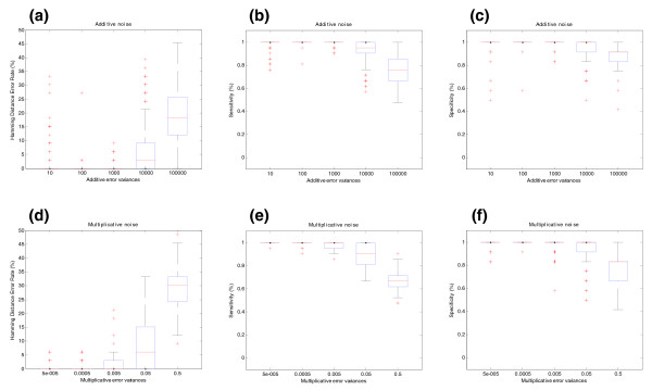
Influence of noise on splicing structure prediction for BIRC5 gene (synthetic data). (a) The effect of additive noise on splicing structure prediction. The y-axis shows the Hamming distance error rate between real and predicted pre-mRNA splicing structures. This measure represents the proportion of probes in a gene that were mistakenly assigned (or unassigned) to each transcript. The units of the x-axis are the variances σ_ε² of the additive error as explained in Figure 1a. (b) Sensitivity of the SPACE algorithm under additive noise. Sensitivity is defined as the proportion of probes that belong to each transcript that are correctly assigned in the predicted structure. (c) Specificity of the SPACE algorithm under additive noise. Specificity is defined as the proportion of probes that do not belong to a particular transcript that are correctly unassigned in the predicted structure. (d) Multiplicative noise effect on splicing structure prediction. The y-axis shows the Hamming distance error rate between real and predicted pre-mRNA splicing structures. The units of the x-axis are the variances σ_η² of the multiplicative error as explained in Figure 1b. (e) Sensitivity of SPACE under multiplicative noise. (f) Specificity of SPACE under multiplicative noise. The Hamming distance error rate is calculated in the form of HD = (FP + FN)/N, the sensitivity is calculated as SN = TP/(TP + FN) and the specificity is calculated as SP = TN/(TN + FP).

Figure 3

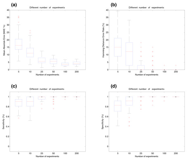
Influence of the number of arrays for BIRC5 gene (synthetic data). (a) Effect of the number of arrays on estimation of relative transcript concentrations. The y-axis shows the MAE (%) between simulated and estimated relative concentration of transcripts. The x-axis shows the different number of arrays used in the simulations. (b) Effect of the number of arrays on splicing structure prediction. The y-axis shows the Hamming Distance Error Rate between real and predicted pre-mRNA splicing structures. (c) Sensitivity of SPACE under different numbers of arrays. (d) Specificity of SPACE under different number of arrays.

Figure 4

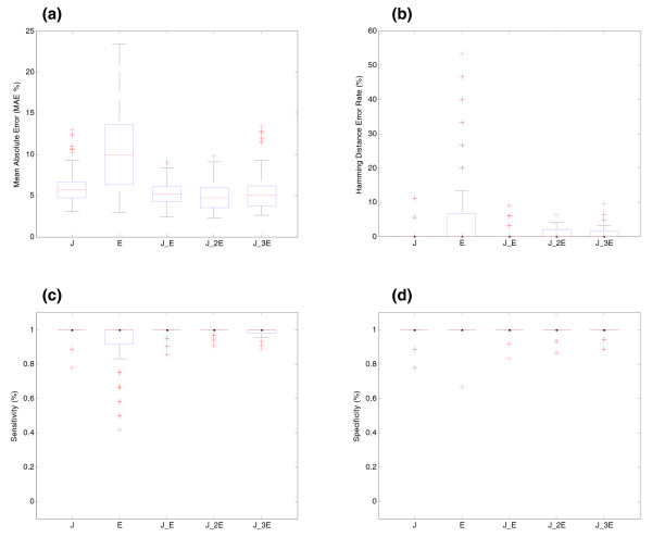
Effect of the location of probes for BIRC5 gene (synthetic data). (a) Effect of the location of the probes on the estimation of relative transcript concentrations. The y-axis shows the MAE (%) between simulated and estimated relative concentration of transcripts. The x-axis shows the different location of probes along the transcripts of the gene. J: the gene is represented by all its junction probes; E: the gene is represented by exon probes located in all its exons; J_E: all junction and exon probes are present in the array; J_2E or J_3E: all junctions and two or three probes per exon, respectively, are present in the array. (b) Effect of the location of the probes on splicing structure prediction. The y-axis shows the Hamming distance error rate between real and predicted pre-mRNA splicing structures. (c) Sensitivity of SPACE with varying location of the probes. (d) Specificity of SPACE with varying location of the probes.

Figure 5

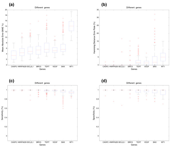
Influence of the gene structure and number of expressed transcripts in a comparative splicing analysis between different genes (synthetic data). (a) Estimation of the relative transcript concentrations for different genes. The y-axis shows the MAE (%) between simulated and estimated relative concentration of transcripts. The x-axis shows the different genes used in the simulation (CASP2, HNRPA2B1, BCL2L1, BIRC5, TERT, VEGF, BAX and WT1). The structure of the different transcripts of these genes and the location of probes is shown in Additional file 1 (Figures S1-S8). (b) Prediction of the splicing structure for different genes. The y-axis shows the Hamming distance error rate between real and predicted pre-mRNA splicing structures. (c) Sensitivity of SPACE for different genes. (d) Specificity of SPACE for different genes.

Figure 6

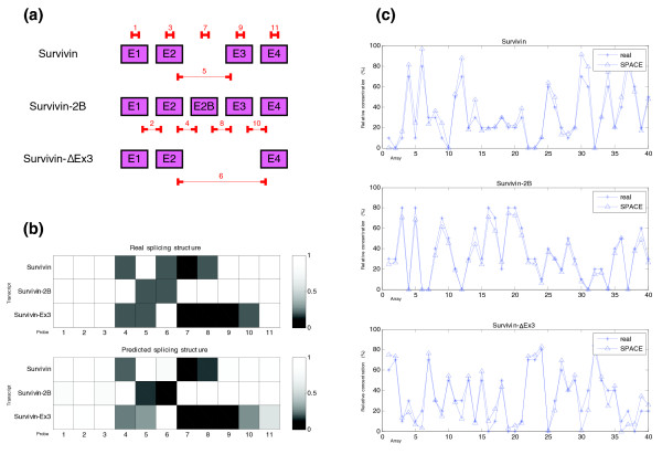
Predicted structure and estimated concentrations for the BIRC5 (apoptosis inhibitor survivin) gene in the 'central point' (synthetic data). (a) Structure of the different transcripts of the BIRC5 gene and location of probes used in the simulation. (b) Representation of the real and predicted splicing structures for the BIRC5 gene given by the probes used. In the graphic representing the real splicing structure the probes that match perfectly with the transcripts are represented by a white box (100% matching) and no hybridization is shown by a black box (0% matching). Gray levels show intermediate matching values. We have assumed that junction probes which include one side of the junction hybridize partially (20%). (c) Estimated relative concentrations of the three isoforms of BIRC5 gene. In each of the three graphics simulated and estimated relative concentration of each isoform is represented.

Figure 7

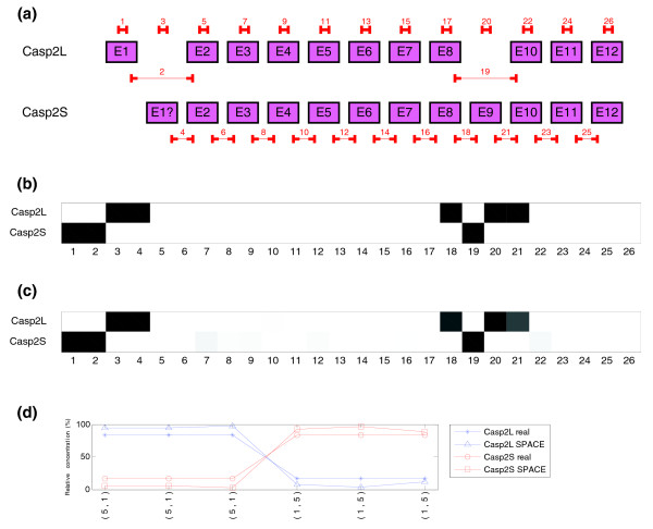
Experiment done with the CASP2 gene, transcripts Casp2L and Casp2S (synthetic data). Three arrays were performed with a concentration ratio between the two isoforms of CASP2 gene equal to 5:1 and another three with the opposite ratio 1:5. (a) Structure of the two transcripts of CASP2 gene and location of probes in the microarray. (b) Real structure of CASP2 gene indicated by probes. Probes that match perfectly are represented in white (100%), no hybridization in black (0%) and partial hybridization by different shades of gray (20%). (c) Predicted splicing structure for CASP2 gene with the alternating concentration ratio 5:1. If compared with the real structure of CASP2 transcripts (b), a strong similarity is noticed. (d) Real and estimated relative concentrations of the two isoforms of CASP2 gene in the experiment.

Figure 8

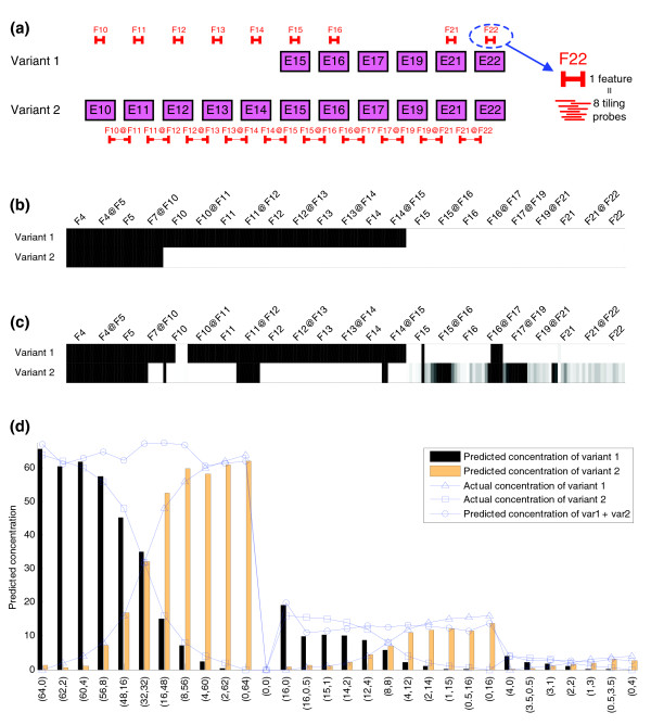
Predicted structure and estimated spiked concentrations for the CD44 gene. (a) Structure of the CD44 gene spiked transcripts and probe positions represented by features. A gene feature is either an exon or a junction. Exon features are represented by F followed by the number of the corresponding exon and junction features are represented by the two exon features to which they belong joined by @ symbol. Each feature is made up of eight probes following a tiling strategy. As 23 features have been measured this makes a total of 184 probes. Probes corresponding to exon features F4, F5 and junction features F4@F5, F7@F10 do not match any of the spiked transcripts and therefore are not shown in (a). (b) Expected hybridization pattern of all probes for each of the two variants of CD44 gene. (c) Splicing structure prediction for CD44 gene applying the SPACE algorithm. (d) Estimated concentrations of the two variants of CD44 gene compared to spiked concentrations. The y-axis shows the predicted and actual concentration of each variant. The x-axis indicates the experiments and actual concentrations of each variant pair.

Figure 9

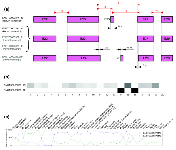
Predicted structure and estimated relative concentrations for the OCRL gene. (a) Structure of the different transcripts (known and novel) of OCRL gene according to Ensembl 40, as well as the real location of the probes in the microarray. As can be seen in the figure, given probes cannot distinguish between a group of three isoforms (one known and two novel). (b) Predicted splicing structure for OCRL gene given by probes. The SPACE algorithm only detect two isoforms that match with known transcripts of OCRL gene ENST00000371113 and ENST0000037112. (c) Estimated relative concentrations of the two isoforms detected of OCRL gene.

Figure 10

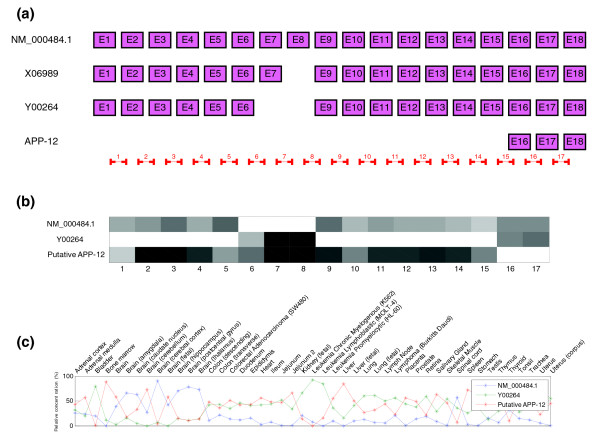
Predicted structure and estimated relative concentrations for the APP gene. (a) Structure of the three different transcripts of the APP gene proposed by Johnson et al. to be present in the samples as well as a short isoform APP-12 that match our results, the real locations of the probes in the microarray are also indicated. (b) Predicted splicing structure for the APP gene given by probes. SPACE detects three isoforms that match with transcripts NM_000484.1, Y00264 and APP-12 of the APP gene. (c) Estimated relative concentrations of the three isoforms detected for the APP gene.

Figure 11

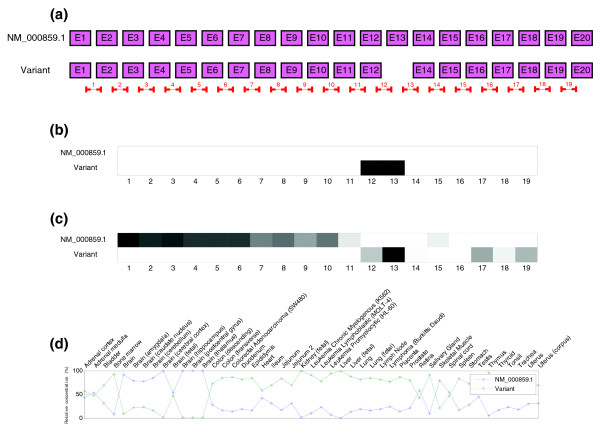
Predicted structure and estimated relative concentrations for the HMGCR gene. (a) Structure of the two transcripts of the HMGCR gene, NM_000859.1 and a variant with a cassette in exon 13, as well as the real locations of the probes in the microarray. (b) Predicted splicing structure for the HMGCR gene given by probes. If compared with the gene structure in (a), it can be seen that the cassette is detected but also more things that do not match with that model. (c) Real and estimated relative concentrations of the two isoforms of HMGCR gene.

Figure 12

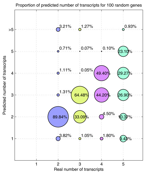
Proportion of predicted number of transcripts for the simulation performed with 100 genes (synthetic data). The 100 genes used have been randomly selected from the human genome with two to five transcripts. Each of the genes have been simulated 200 times for different noise, concentrations and affinities. The area of each circle represents the proportion of times the corresponding predicted number is chosen by the algorithm for a given number of transcripts. The algorithm tends to underestimate the number of transcripts as the real number of transcripts increases.

Figure 13

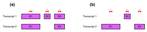
Example of the non-uniqueness of the splicing structure prediction. (a) Structure of a generic gene and proposed probe pattern. (b) Possible splicing structure prediction obtained by SPACE with the same probe pattern.